"tinyBenchmarks:用更少样本评测大语言模型"
"tinyBenchmarks: evaluating LLMs with fewer examples"
推荐全译对照查看原文(PDF) ↗
导读
本文属于第 7 周「评测基础」单元,讨论一个非常现实的问题:基准越来越大,评测越来越贵——Liang 等人报告在 HELM 上评测一个 LLM 花费超过 4,000 GPU 小时(API 则超 1 万美元),而预训练期间的检查点监控、提示策略与超参探索又要求反复评测。作者 Felipe Maia Polo 等(密歇根大学统计系、IBM Research、MIT 等,ICML 2024)给出的答案是:借助心理测量学(psychometrics)中几十年成熟的项目反应理论(Item Response Theory, IRT)——GRE、SAT 等标准化考试背后的统计模型——把 LLM 视为「考生」、基准题目视为「试题」,从历史评测数据中学习每道题的难度与所需能力,进而选出少数最有信息量的「锚点」题目。
核心结论令人印象深刻:估计一个 LLM 在 MMLU(约 14,000 题)上的真实准确率,只需在 100 道精选题上评测,平均误差约 2%——评测成本降低 140 倍。论文发布了 Open LLM Leaderboard、MMLU、HELM、AlpacaEval 2.0 的 tiny 版本与基于 IRT 的估计工具(CPU 数秒即可运行),对频繁评测场景(微调、提示工程、基准加速)极其实用。它与 Press 的基准设计帖互补:一个讲「怎么造好基准」,一个讲「怎么便宜地用好基准」,也为理解后续 Agent 基准的成本问题提供了统计工具箱。
全文对照翻译
译注:以下覆盖论文正文全部内容(标题作者、摘要、第 1–6 节含 6.1 扩展与 6.2 局限、致谢、影响声明,原文第 1–9 页),以及附录 A–E 的实质内容(平衡权重、tinyMMLU 分析、命题 4.1 证明、基准补充细节、额外结果);附录 F(图 17–32,逐场景误差图)仅含图题、无正文文字,以译注概述;References 不收录。原文脚注以「(原文脚注 N:……)」形式并入相应位置;公式以 LaTeX 重排、编号与原文一致。术语首现处中英对照:项目反应理论(Item Response Theory, IRT)、锚点(anchor point)、分层随机抽样(stratified random sampling)、正确性(correctness)、场景(scenario)、示例(example)、变分推断(variational inference)、有效样本量(effective sample size, ESS)、分布偏移(distribution shift)、维度灾难(curse of dimensionality)、自适应测试(adaptive testing)、主动测试(active testing)等。
题目与作者
tinyBenchmarks: evaluating LLMs with fewer examples
Felipe Maia Polo 1 Lucas Weber 2 Leshem Choshen 3 4 Yuekai Sun 1 Gongjun Xu 1 Mikhail Yurochkin 3 5
1Department of Statistics, University of Michigan, USA
2Department of Translation and Language Sciences, University of Pompeu Fabra, Spain 3IBM Research 4MIT 5MIT-IBM Watson AI Lab. Correspondence to: Felipe Maia Polo <felipemaiapolo@gmail.com>.
Proceedings of the 41st International Conference on Machine Learning, Vienna, Austria. PMLR 235, 2024. Copyright 2024 by the author(s).
tinyBenchmarks:用更少示例评测大语言模型。作者:Felipe Maia Polo、Lucas Weber、Leshem Choshen、Yuekai Sun、Gongjun Xu、Mikhail Yurochkin,分别来自密歇根大学统计系、庞培法布拉大学翻译与语言科学系、IBM Research、MIT 与 MIT-IBM Watson AI Lab。发表于第 41 届国际机器学习会议(ICML 2024,奥地利维也纳,PMLR 235)。(原文脚注:通讯作者 felipemaiapolo@gmail.com;原文脚注 1:要用我们的方法高效评测 LLM,请查看 https://github.com/felipemaiapolo/tinyBenchmarks——该仓库含一个用于模型评测的 Python 包与教程;此外我们已把 tiny 数据集上传至 huggingface.co/tinyBenchmarks,并制作了一个 Google Colab 演示,可便捷地用我们的工具估计 LLM 在 MMLU 上的性能;复现本文结果请查看该 GitHub 仓库。)
摘要(Abstract)
The versatility of large language models (LLMs) led to the creation of diverse benchmarks that thoroughly test a variety of language models' abilities. These benchmarks consist of tens of thousands of examples making evaluation of LLMs very expensive. In this paper, we investigate strategies to reduce the number of evaluations needed to assess the performance of an LLM on several key benchmarks. For example, we show that to accurately estimate the performance of an LLM on MMLU, a popular multiple-choice QA benchmark consisting of 14K examples, it is sufficient to evaluate this LLM on 100 curated examples. We release evaluation tools and tiny versions of popular benchmarks: Open LLM Leaderboard, MMLU, HELM, and AlpacaEval 2.0. Our empirical analysis demonstrates that these tools and tiny benchmarks are sufficient to reliably and efficiently reproduce the original evaluation results.
大语言模型(LLM)的多才多艺催生了多样的基准(benchmark),用以全面测试各种语言模型的能力。这些基准由数万个示例(example)组成,使得对 LLM 的评测非常昂贵。本文研究能减少「在若干关键基准上评估 LLM 性能」所需评测次数的策略。例如,我们证明:要准确估计一个 LLM 在流行选择题问答基准 MMLU(由 14K 个示例组成)上的性能,只需在该 LLM 上评测 100 个精选(curated)示例即可。我们发布评测工具以及流行基准的 tiny 版本:Open LLM Leaderboard、MMLU、HELM 与 AlpacaEval 2.0。我们的实证分析表明,这些工具与 tiny 基准足以可靠且高效地复现原始评测结果。
1 引言(Introduction)
Large Language Models (LLMs) have demonstrated remarkable abilities to solve a diverse range of tasks (Brown et al., 2020). Quantifying these abilities and comparing different LLMs became a challenge that led to the development of several key benchmarks, e.g., MMLU (Hendrycks et al., 2020), Open LLM Leaderboard (Beeching et al., 2023), HELM (Liang et al., 2022), and AlpacaEval (Li et al., 2023). These benchmarks are comprised of hundreds or thousands of examples, making the evaluation of modern LLMs with billions of parameters computationally, environmentally, and financially very costly. For example, Liang et al. (2022) report that evaluating the performance of a single LLM on HELM costs over 4K GPU hours (or over $10K for APIs). Benchmarks like AlpacaEval (Li et al., 2023) also require a commercial LLM as a judge to perform evaluation, further increasing the costs. Furthermore, evaluation of a single model is often performed many times to monitor checkpoints during pre-training (Biderman et al., 2023a; Liu et al., 2023) and to explore different prompting strategies or a wider range of hyperparameters (Weber et al., 2023b; Mizrahi et al., 2023; Sclar et al., 2023; Voronov et al., 2024).
大语言模型(LLM)已展现出解决多样任务的卓越能力(Brown et al., 2020)。量化这些能力并比较不同的 LLM 成为一项挑战,并催生了若干关键基准,例如 MMLU(Hendrycks et al., 2020)、Open LLM Leaderboard(Beeching et al., 2023)、HELM(Liang et al., 2022)与 AlpacaEval(Li et al., 2023)。这些基准包含成百上千乃至上万个示例,使得对拥有数十亿参数的现代 LLM 的评测在算力、环境与财务上都非常昂贵。例如,Liang et al. (2022) 报告:在 HELM 上评测单个 LLM 的性能花费超过 4K GPU 小时(若用 API 则超过 1 万美元)。AlpacaEval(Li et al., 2023)这类基准还需要一个商用 LLM 作为裁判(judge)来执行评测,进一步推高成本。此外,对单个模型的评测往往要进行很多次:预训练期间监控检查点(Biderman et al., 2023a; Liu et al., 2023),以及探索不同提示策略或更大范围的超参数(Weber et al., 2023b; Mizrahi et al., 2023; Sclar et al., 2023; Voronov et al., 2024),都要求反复评测。
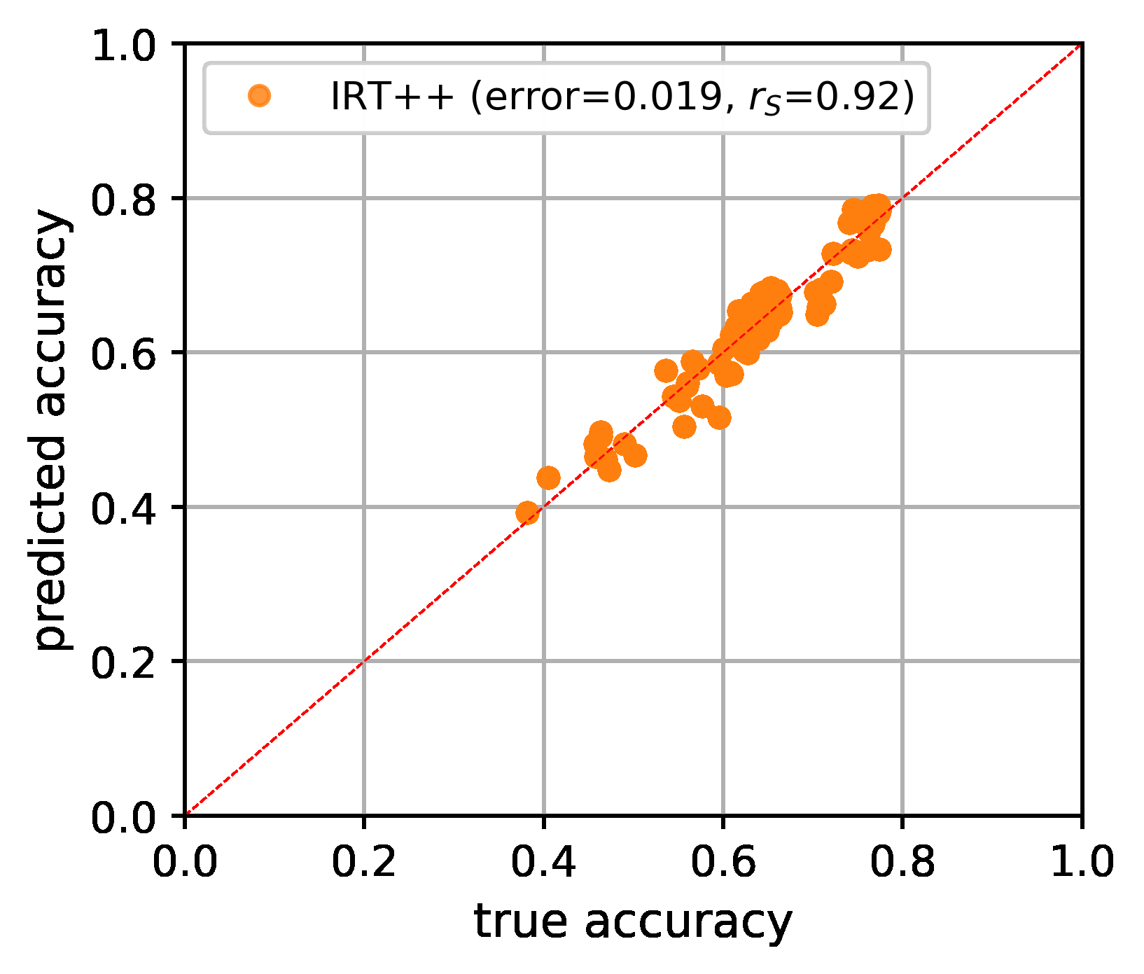
[图 1: Estimating accuracy on MMLU (true accuracy) using 100 curated examples (predicted accuracy). IRT++, our best-performing evaluation strategy, predicts the accuracy of recent LLMs released between December 30th and January 18th within 1.9% of their true accuracy on all of MMLU (14K examples).]
图 1:用 100 道精选示例估计 MMLU 上的准确率——纵轴为预测准确率、横轴为真实准确率,每个点是一个 LLM。我们表现最好的评测策略 IRT++ 在预测 2023 年 12 月 30 日至 2024 年 1 月 18 日之间发布的近期 LLM 的准确率时,与它们在全部 MMLU(14K 示例)上的真实准确率相差不超过 1.9%。
Our work reassesses the need to evaluate LLMs on such large benchmark datasets. In Figure 1 we demonstrate the efficacy of our best evaluation strategy on MMLU, where we compare accuracy estimates obtained from evaluating LLMs on a curated subset of 100 examples (less than 1% of the examples) to accuracy on all of MMLU, achieving average estimation error under 2%.
我们的工作重新审视了「必须在这类大型基准数据集上评测 LLM」的必要性。图 1 展示了我们的最佳评测策略在 MMLU 上的效果:我们把「在 100 个精选示例(不足全部示例的 1%)上评测 LLM 所得准确率估计」与「全部 MMLU 上的准确率」进行比较,平均估计误差低于 2%。
We consider a range of evaluation strategies (§3):
1. Stratified random sampling as proposed by Perlitz et al. (2023) for HELM. This approach is the simplest to use but can result in a large estimation error.
2. Clustering examples based on LLMs that have already been evaluated. The key idea is to find examples where (in)correct prediction of an LLM implies that it will also be (in)correct on a subset of other examples. This method performs well in some settings but can be unreliable when such correctness patterns are spurious, e.g., when predicting the accuracy of an LLM specialized to a domain. This strategy is inspired by the Anchor Points method (Vivek et al., 2023) which clusters models' confidence in the correct class for faster evaluation on classification tasks.
3. New strategies built using Item Response Theory (IRT) (Lord et al., 1968) for evaluating individuals through standardized tests. Applying IRT to LLMs viewed as testees and benchmarks as tests, we learn representations of examples encoding latent abilities required to perform well on these examples. Clustering these representations allows us to find a more robust evaluation set. Furthermore, using the IRT model, we develop tools for improving benchmark accuracy estimates obtained with an arbitrary set of examples.
我们考虑一系列评测策略(§3):
-
Perlitz et al. (2023) 为 HELM 提出的分层随机抽样(stratified random sampling)。这种方法用起来最简单,但可能带来较大的估计误差。
-
基于已被评测过的 LLM 对示例做聚类(clustering)。关键想法是找出这样一些示例:LLM 对它们的(不)正确预测,蕴含着它对另一子集示例也将(不)正确。该方法在某些设定下表现良好,但当这种正确性模式(correctness patterns)是伪相关(spurious)时可能不可靠,例如在预测某个领域特化 LLM 的准确率时。该策略受锚点(Anchor Points)方法(Vivek et al., 2023)启发——后者聚类模型对正确类别的置信度,以加速分类任务上的评测。
-
使用项目反应理论(Item Response Theory, IRT)(Lord et al., 1968)构建的新策略;IRT 是通过标准化测试评测个体的理论。把 LLM 视为考生、基准视为试卷来应用 IRT,我们学习到的示例表示编码了在这些示例上取得好成绩所需的潜在能力(latent abilities)。对这些表示进行聚类让我们得到更鲁棒的评测集。此外,借助 IRT 模型,我们还开发了改进「用任意示例集得到的基准准确率估计」的工具。
We present an extensive evaluation of these strategies on four popular benchmarks (§5): Open LLM Leaderboard (Beeching et al., 2023), MMLU (Hendrycks et al., 2020), HELM (Liang et al., 2022), and AlpacaEval 2.0 (Li et al., 2023). Our goal is to assess the effectiveness of estimating the performance of LLMs on these benchmarks using a limited number of examples for evaluation. Overall, we conclude that 100 curated examples per scenario are enough to reliably estimate the performance of various LLMs, within about 2% error on average. Based on our findings we release tiny (100 examples per scenario) versions of every considered benchmark and IRT-based tools for further improving the performance estimation.
我们在四个流行基准(§5)上对这些策略进行了广泛评测:Open LLM Leaderboard(Beeching et al., 2023)、MMLU(Hendrycks et al., 2020)、HELM(Liang et al., 2022)与 AlpacaEval 2.0(Li et al., 2023)。我们的目标是评估:用有限数量的评测示例估计 LLM 在这些基准上的性能,效果如何。总体而言,我们的结论是:每场景 100 个精选示例就足以可靠地估计各种 LLM 的性能,平均误差约 2%。基于这些发现,我们发布了每个所考虑基准的 tiny 版本(每场景 100 个示例),以及用于进一步改进性能估计的基于 IRT 的工具。
1.1 相关工作(Related work)
Efficient benchmarking of LLMs Multi-dataset benchmarks were introduced to the field of NLP with the advent of pre-trained models (e.g. Wang et al., 2018), and constantly evolved in lockstep with language model capabilities (Srivastava et al., 2022). The ever-increasing size of models and datasets consequently led to high evaluation costs, triggering changes in reported evaluation to accommodate the costs (Biderman et al., 2023b). Ye et al. (2023) considered reducing the number of tasks in Big-bench (Srivastava et al., 2022). Perlitz et al. (2023) found that evaluation on HELM (Liang et al., 2022) relies on diversity across datasets, but the number of examples currently used is excessive. We adopt their stratified sampling approach as one of the efficient evaluation strategies. Vivek et al. (2023) proposed clustering evaluation examples based on models' confidence in the correct class for faster evaluation on classification tasks. One of the approaches we consider is based on an adaptation of their method to popular LLM benchmarks with more diverse tasks.
LLM 的高效评测(efficient benchmarking)。多数据集基准随预训练模型的出现被引入 NLP 领域(如 Wang et al., 2018),并与语言模型能力同步不断演进(Srivastava et al., 2022)。模型与数据集规模的持续增长随之带来高昂的评测成本,促使论文所报告的评测方式做出调整以适应成本(Biderman et al., 2023b)。Ye et al. (2023) 考虑过缩减 Big-bench(Srivastava et al., 2022)的任务数量。Perlitz et al. (2023) 发现 HELM(Liang et al., 2022)上的评测依赖跨数据集的多样性,但当前使用的示例数量过多。我们采纳他们的分层抽样方法作为高效评测策略之一。Vivek et al. (2023) 提出按模型对正确类别的置信度聚类评测示例,以加速分类任务上的评测。我们考虑的方法之一,正是把他们的方法改造后应用到任务更加多样的流行 LLM 基准上。
Item response theory (IRT) IRT (Cai et al., 2016; Van der Linden, 2018; Brzezińska, 2020; Lord et al., 1968) is a well-established set of statistical models used in psychometrics to measure the latent abilities of individuals through standardized testing (An & Yung, 2014; Kingston & Dorans, 1982; Petersen et al., 1982), e.g., in GRE, SAT, etc.. Even though IRT methods have been traditionally used in psychometrics, they are becoming increasingly popular among researchers in the fields of artificial intelligence and natural language processing (NLP). For instance, Lalor et al. (2016) propose using IRT's latent variables to measure language model abilities, Vania et al. (2021) employs IRT models in the context of language models benchmarking to study saturation (un-discriminability) of commonly used benchmarks, and Rodriguez et al. (2021) study several applications of IRT in the context of language models, suggesting that IRT models can be reliably used to: predict responses of LLMs in unseen items, categorize items (e.g., according to their difficulty/discriminability), and rank models. More recently, Zhuang et al. (2023) used IRT for adaptive testing, making testing more efficient. However, the authors do not propose a performance estimator for LLMs but only rank models based on their ability parameters. To the best of our knowledge, IRT has not been used for performance estimation in the context of efficient benchmarking of LLMs. We explore this new path.
项目反应理论(IRT)。IRT(Cai et al., 2016; Van der Linden, 2018; Brzezińska, 2020; Lord et al., 1968)是心理测量学(psychometrics)中一整套成熟的统计模型,通过标准化测试度量个体的潜在能力(An & Yung, 2014; Kingston & Dorans, 1982; Petersen et al., 1982),例如 GRE、SAT 等考试背后的模型。尽管 IRT 方法传统上用于心理测量学,它在人工智能与自然语言处理(NLP)领域的研究者中正变得日益流行。例如,Lalor et al. (2016) 提出用 IRT 的潜变量度量语言模型能力;Vania et al. (2021) 在语言模型基准评测的语境中应用 IRT 模型,研究常用基准的饱和(不可区分性)问题;Rodriguez et al. (2021) 研究了 IRT 在语言模型语境中的多种应用,提示 IRT 模型可被可靠地用于:预测 LLM 在未见题目上的回答、对题目分类(如按难度/区分度)、以及对模型排序。更近的 Zhuang et al. (2023) 用 IRT 做自适应测试(adaptive testing),使测试更高效;但作者并未提出面向 LLM 的性能估计器,只是基于能力参数对模型排序。据我们所知,IRT 尚未在「LLM 高效基准评测」的语境中被用于性能估计。我们探索了这条新路径。
Active testing Another line of related work is related to active learning (Ein-Dor et al., 2020) and especially active testing. In such works, evaluation examples are chosen dynamically using various criteria (Ji et al., 2021; Kossen et al., 2021; Zhuang et al., 2023) to minimize annotation costs. Those methods are somewhat similar to the adaptive IRT which we discuss in §6.
主动测试(active testing)。另一条相关工作线索与主动学习(active learning)(Ein-Dor et al., 2020)、尤其是主动测试相关。这类工作使用多种准则动态选择评测示例(Ji et al., 2021; Kossen et al., 2021; Zhuang et al., 2023),以最小化标注成本。这些方法与我们在 §6 讨论的自适应 IRT 有些相似。
2 问题设定(Problem statement)
In this section, we describe in detail the setup we work on and what are our objectives. Consider that a benchmark is composed of scenarios and possibly sub-scenarios. For example, MMLU and HellaSwag are examples of scenarios of both the Open LLM Leaderboard and HELM, while MMLU has different sub-scenarios like "marketing", "elementary mathematical", and so on. Furthermore, each scenario (or sub-scenario) is composed of examples (analogous to "items" in the IRT literature) that are small tests to be solved by the LLMs–these examples range from multiple-choice questions to text summarization tasks.
本节详细描述我们工作的设定与目标。设想一个基准由若干场景(scenario)组成,场景下还可能有子场景(sub-scenario)。例如,MMLU 与 HellaSwag 既是 Open LLM Leaderboard 也是 HELM 的场景,而 MMLU 又有「市场营销」「初等数学」等不同子场景。进一步,每个场景(或子场景)由示例(example)构成(类比 IRT 文献中的「项目/item」),即需要 LLM 去完成的小测试——这些示例从多选题到文本摘要任务不一而足。(原文脚注 2:我们把 MMLU 与 AlpacaEval 各视为单一场景。)
Our final objective is to estimate the performance of LLMs in the full benchmark, which is given by the average of the performances in individual scenarios (Open LLM Leaderboard, MMLU, AlpacaEval 2.0) or mean-win-rate (HELM). We achieve this objective by first estimating the performance of LLMs in individual scenarios and then aggregating scores. When scenarios have sub-scenarios, it is usually the case that the scenario performance is given by a simple average of sub-scenarios performances. The main concern is that each scenario/sub-scenario is composed of hundreds or thousands of examples, making model evaluation costly.
我们的最终目标是估计 LLM 在整个基准上的性能,它由各场景性能的平均给出(Open LLM Leaderboard、MMLU、AlpacaEval 2.0),或由平均胜率(mean-win-rate)给出(HELM)。我们先估计 LLM 在各场景的性能、再汇总得分,以此达成该目标。当场景有子场景时,场景性能通常由各子场景性能的简单平均给出。主要的顾虑在于:每个场景/子场景由成百上千个示例组成,使模型评测代价高昂。
In this work, for a fixed benchmark, we denote the set of examples of each scenario j as Ij, implying that the totality of examples in the benchmark is given by I = ∪j Ij. When an LLM l interacts with an example i ∈ I j, the system behind the benchmarks generates a score that we call "correctness" and denote as Yil. In all the benchmarks we consider in this work, the correctness is either binary, i.e., Yil ∈ {0, 1} (incorrect/correct), or bounded, i.e., Yil ∈ [0, 1], denoting a degree of correctness. The second case is applied in situations in which, for instance, there might not be just one correct answer for example i. To simplify the exposition in the text, we assume that the score for LLM l in scenario j is just the simple average of the correctness of all items in that scenario, that is, 1/|Ij| Σi∈Ij Yil. That is not true when different sub-scenarios have different numbers of examples; in that case, one would just have to use a weighted average instead, to make sure every sub-scenario is equally important (in the experiments, we consider this case).
本文中,对一个固定基准,我们把场景 $j$ 的示例集记为 $I_j$,于是基准的全部示例为 $I = \bigcup_j I_j$。当 LLM $l$ 与示例 $i \in I_j$ 交互时,基准背后的系统产生一个我们称为「正确性(correctness)」的得分,记作 $Y_{il}$。在本文考虑的所有基准中,正确性要么是二值的,即 $Y_{il} \in \{0, 1\}$(错误/正确);要么是有界的,即 $Y_{il} \in [0, 1]$,表示某种正确程度。第二种情形适用于诸如示例 $i$ 可能不止一个正确答案的情况。为行文简洁,我们假设 LLM $l$ 在场景 $j$ 的得分就是该场景全部项目正确性的简单平均,即 $\frac{1}{|I_j|}\sum_{i \in I_j} Y_{il}$。当不同子场景的示例数不同时该假设不成立;那种情形下只需改用加权平均,以保证每个子场景同等重要(实验中我们考虑了这种情形)。
Our objective is to choose a small fraction of examples Îj ⊂ I j such that we can estimate score of a new LLM l, i.e., 1/|Ij| Σi∈Ij Yil, using its correctness evaluated only on the examples in Îj ⊂ I j, i.e., {Yil}i∈Îj. To intelligently choose Îj we assume access to correctness evaluations for a set of LLMs that have been previously evaluated on the entirety of the benchmark. Such correctness data is freely available for many popular benchmarks. In the next section, we describe strategies on how Îj can be chosen and how the LLMs performance on the full benchmark can be estimated.
我们的目标是选出示例的一小部分 $\hat I_j \subset I_j$,使得我们能仅用新 LLM $l$ 在 $\hat I_j \subset I_j$ 上评测得到的正确性,即 $\{Y_{il}\}_{i \in \hat I_j}$,来估计它在场景上的得分,即 $\frac{1}{|I_j|}\sum_{i \in I_j} Y_{il}$。为聪明地选出 $\hat I_j$,我们假设能拿到一组「已在整个基准上被评测过」的 LLM 的正确性评测数据。这类正确性数据对许多流行基准都是免费公开的。下一节将描述如何选择 $\hat I_j$,以及如何估计 LLM 在完整基准上的性能。
3 选择评测示例(Selecting evaluation examples)
In this section, we describe strategies on how to select examples from a fixed scenario j, i.e., Ij, obtaining Îj ⊂ I j described in Section 2. Ideally, the set of selected examples should be representative of the whole set of items in scenario j, that is,
Σi∈Îj wiYil ≈ 1/|Ij| Σi∈Ij Yil, (3.1)
for nonnegative weights {wi}i∈Îj such that Σi∈Îj wi = 1. In the next paragraphs, we describe two possible ways of obtaining Îj and {wi}i∈Îj.
本节描述如何从固定场景 $j$(即 $I_j$)中选择示例,得到第 2 节所述的 $\hat I_j \subset I_j$。理想情况下,所选示例集应能代表场景 $j$ 的全部题目,即
其中权重 $\{w_i\}_{i\in\hat I_j}$ 非负且 $\sum_{i\in\hat I_j} w_i = 1$。下面各段描述得到 $\hat I_j$ 与 $\{w_i\}_{i\in\hat I_j}$ 的两种可行方式。
3.1 分层随机抽样(Stratified random sampling)
In some settings (e.g., classifiers Katariya et al., 2012), it is useful to perform stratified random sampling – subsample examples ensuring the representation of certain groups of data. Using subscenarios as the strata for stratified random sampling was proposed by Perlitz et al. (2023) when subsampling examples from HELM scenarios. The authors showed that this is an effective way of sampling examples without too much loss on the ability to rank LLMs by performance. Examples should be randomly selected from sub-scenarios (with uniform probability) in a way such that the difference in number of examples sampled for two distinct subscenarios is minimal (≤ 1). The rationale behind this method is that, for an effective evaluation, sub-scenarios should be equally represented. The weights are wi = 1/|Îj| for all i ∈ Îj.
在某些设定下(如分类器,Katariya et al., 2012),执行分层随机抽样很有用——即采样子示例时保证特定数据组别得到代表。以子场景为层(strata)做分层随机抽样,由 Perlitz et al. (2023) 在从 HELM 场景下采样示例时提出。作者表明这是一种有效的示例采样方式,且不太损失按性能对 LLM 排序的能力。示例应以均匀概率从各子场景随机抽取,并使任意两个不同子场景被抽到的示例数之差最小(≤ 1)。该方法背后的道理是:一次有效的评测应让各子场景得到同等代表。权重取 $w_i = 1/|\hat I_j|$,$\forall i \in \hat I_j$。
3.2 聚类(Clustering)
Assessing the performance of LLM's on a randomly sampled subset of examples suffers from extra uncertainty in the sampling process, especially when the number of sampled examples is small. Instead, we consider selecting a subset of representative examples using clustering. Vivek et al. (2023) proposed to cluster examples based on the confidence of models in the correct class corresponding to these examples. Representative examples, from these clusters, which they call "anchor points", can then be used to evaluate models on classification tasks more efficiently. We adapt their clustering approach to a more general setting, allowing us to extract such anchor points for MMLU, AlpacaEval 2.0, and all scenarios of the Open LLM Leaderboard and HELM.
在随机采样的示例子集上评测 LLM 的性能,会额外承受采样过程的不确定性,当采样示例数少时尤甚。作为替代,我们考虑用聚类(clustering)选择一组代表性示例。Vivek et al. (2023) 提出按模型对这些示例所对应正确类别的置信度来聚类示例;从这些簇中得到的代表性示例——他们称之为「锚点(anchor points)」——随后可用于更高效地在分类任务上评测模型。我们把他们的聚类方法适配到更一般的设定,使我们可以为 MMLU、AlpacaEval 2.0 以及 Open LLM Leaderboard 与 HELM 的全部场景提取此类锚点。
First, we propose to group examples by model correctness, expecting some examples would represent the rest. Ideally, if example i is an anchor point, then there will be a big set of examples on which models are correct if and only if they get example i correct. The same idea applies when correctness is given by a number in [0, 1]. Assume that we want to select K anchor points and have access to the training set Dtr = {Yl}l∈Ltr, where Yl is a vector in which each entry is given by the correctness score Yil for all examples i ∈ I j. We represent each example i ∈ I j by the embedding Ei ∈ R|Ltr| which is a vector with entries given by Yil for l ∈ Ltr, and then run K-Means (Hastie et al., 2009) with the number of clusters being equal K. After the K centroids are obtained, we find the closest example to each centroid, and each of those points will compose Îj. For a new LLM l ∉ Ltr to be evaluated, we can obtain an estimate for its performance using the estimate in equation 3.1 by setting wi as the fraction of points in Ij assigned to cluster/anchor point i. This method is compelling and simple in detecting anchor points. Still, it can suffer from distribution shifts since correctness patterns can vary, e.g., in time, and from the curse of dimensionality when |Ltr| is big. Our second approach is intended to be more robust to those problems.
第一种做法,我们提出按模型正确性对示例分组,期望某些示例能代表其余示例。理想情况下,若示例 $i$ 是锚点,则应存在一大组示例,模型们「当且仅当做对了示例 $i$ 才做对那组示例」。正确性取值为 $[0,1]$ 中的数时,同样的想法也适用。设我们要选 $K$ 个锚点,并能访问训练集 $\mathcal{D}_{tr} = \{Y_l\}_{l \in \mathcal{L}_{tr}}$,其中 $Y_l$ 是一个向量,各元素为示例 $i \in I_j$ 上的正确性得分 $Y_{il}$。我们把每个示例 $i \in I_j$ 表示为嵌入(embedding)$E_i \in \mathbb{R}^{|\mathcal{L}_{tr}|}$——其各元素为 $l \in \mathcal{L}_{tr}$ 各 LLM 的 $Y_{il}$——然后以簇数等于 $K$ 运行 K-Means(Hastie et al., 2009)。得到 $K$ 个质心(centroid)后,我们找出离每个质心最近的示例,这些点即组成 $\hat I_j$。对要评测的新 LLM $l \notin \mathcal{L}_{tr}$,我们把 $w_i$ 设为 $I_j$ 中被分配给簇/锚点 $i$ 的点的比例,即可用式 3.1 得到其性能估计。该方法在检测锚点上很有说服力且简单,但仍有两点隐患:正确性模式可能随时间等变化而带来分布偏移(distribution shift);以及当 $|\mathcal{L}_{tr}|$ 大时的维度灾难(curse of dimensionality)。我们的第二种方法旨在对这两个问题更鲁棒。
The second approach we propose is using item response theory (IRT) representation of examples, detailed in Section 4, as our embeddings Ei. The IRT model creates a meaningful representation for each example i based on their difficulty and the abilities required to respond to those examples correctly. This approach immediately solves the dimensionality problem, since Ei is relatively low-dimensional, and potentially alleviates the distribution shift problem if the IRT model reasonably describes the reality and the example representations are stable. As IRT should represent which examples have similar difficulty and require similar abilities, the anchors represent exactly what we looked for. The weight wi is given by the fraction of examples in Ij assigned to cluster/anchor point i.
我们提出的第二种方法,是用第 4 节详述的示例的项目反应理论(IRT)表示作为嵌入 $E_i$。IRT 模型基于每个示例 $i$ 的难度与正确作答它所需的能力,为其创建有意义的表示。该方法立即解决了维度问题($E_i$ 相对低维;原文脚注 3:实验中 $E_i$ 的维度 ≤ 16),并且若 IRT 模型合理地描述了现实、示例表示保持稳定,它还可能缓解分布偏移问题。由于 IRT 本应刻画「哪些示例难度相近、所需能力相近」,这样得到的锚点恰好代表我们想要找的东西。权重 $w_i$ 由分配给簇/锚点 $i$ 的 $I_j$ 中示例的比例给出。
4 用 IRT 改进性能估计(Better performance estimation with IRT)
In this section, we propose ways of enhancing performance estimates by using IRT models. We start by discussing the case where Yil ∈ {0, 1}, that is, the l responds to the example i ∈ I correctly or not. We later also discuss the case where Yil ∈ [0, 1].
本节提出用 IRT 模型增强性能估计的若干途径。我们先讨论 $Y_{il} \in \{0, 1\}$ 的情形,即 LLM $l$ 答对示例 $i \in I$ 与否;随后也讨论 $Y_{il} \in [0, 1]$ 的情形。
4.1 IRT 模型(The IRT model)
The two-parameter multidimensional IRT model assumes that the probability of the LLM j getting example i correctly is given by
pil ≜ P(Yil = 1|θl,αi,βi) = 1 / (1+exp(−α⊤i θl+βi)), (4.1)
where θl ∈ Rd denotes the unobserved abilities of LLM l, while αi ∈ Rd dictates which dimensions of θl are required from model l to respond to example i correctly. In this formulation, βi ∈ R can be viewed as a bias term that regulates the probability of correctness when θl = 0. We use IRT parameter estimates as example representations referred to in Section 3. Specifically, we take Ei = (α̂i, β̂i), where α̂i and β̂i are point estimates for the parameters of example i. In the next sections, we introduce two estimators for the performance of an LLM, propose a simple solution for the case Yil ∉ {0, 1}, and describe model fitting.
两参数多维 IRT 模型(two-parameter multidimensional IRT model)假设 LLM 答对示例 $i$ 的概率为(译注:原文此处写作「LLM j」,系原文记号笔误,其余各处均以 $l$ 指代 LLM):
其中 $\theta_l \in \mathbb{R}^d$ 表示 LLM $l$ 的不可观测能力(abilities),而 $\alpha_i \in \mathbb{R}^d$ 指明模型 $l$ 要答对示例 $i$ 需要动用 $\theta_l$ 的哪些维度。在这一表述中,$\beta_i \in \mathbb{R}$ 可视为一个偏置(bias)项,在 $\theta_l = 0$ 时调节答对的概率。我们用 IRT 参数估计作为第 3 节所说的示例表示:具体地,取 $E_i = (\hat\alpha_i, \hat\beta_i)$,其中 $\hat\alpha_i$ 与 $\hat\beta_i$ 是示例 $i$ 参数的点估计(point estimates)。接下来几个小节,我们介绍两个 LLM 性能估计器,为 $Y_{il} \notin \{0, 1\}$ 的情形提出一个简单解法,并描述模型拟合。
4.2 基于 IRT 的 LLM 性能估计(IRT-based LLM performance estimation)
The performance-IRT (p-IRT) estimator. Assume that we are interested in estimating the performance of a model l ∉ Ltr on scenario j and that point estimates of example parameters, (α̂i, β̂i), have been computed, using a training set, for all examples in all scenarios, including examples i ∈ I j. Formally, we are interested in approximating
Zjl ≜ 1/|Ij| Σi∈Ij Yil (4.2)
性能-IRT(p-IRT)估计器。假设我们想估计模型 $l \notin \mathcal{L}_{tr}$ 在场景 $j$ 上的性能,且已用某个训练集为所有场景的全部示例(包括 $I_j$ 中的示例 $i$)算出了示例参数的点估计 $(\hat\alpha_i, \hat\beta_i)$。形式上,我们想逼近
Now, assume that we have run model l on a subset of examples from scenario j, obtaining responses {Yi0l,··· ,Yikl} for the examples Îj = {i0,··· ,ik}. Let θ̂l denote the estimate for θl after observing Îj and possibly a bigger set of examples coming from different scenarios. To obtain that estimate, we maximize the log-likelihood of the freshly observed data with respect to θl, fixing examples' parameters. This procedure is equivalent to fitting a logistic regression model, which is an instance of the well-studied M-estimation procedure.
现在,假设我们已让模型 $l$ 在场景 $j$ 的一个示例子集上作答,得到示例 $\hat I_j = \{i_0, \dots, i_k\}$ 上的回答 $\{Y_{i_0 l}, \dots, Y_{i_k l}\}$。令 $\hat\theta_l$ 表示在观察到 $\hat I_j$、以及可能来自不同场景的更大示例集之后对 $\theta_l$ 的估计。为得到该估计,我们在固定示例参数的条件下,对 $\theta_l$ 最大化新观测数据的对数似然。该过程等价于拟合一个逻辑回归(logistic regression)模型——它是被充分研究过的 M-估计(M-estimation)程序的一个实例。
Because Zjl is a random variable, we approximate it by estimating the conditional expectation
E[Zjl|Yi0l,··· ,Yikl] = 1/|Ij| Σi∈Ij E[Yil|Yi0l,··· ,Yikl] = 1/|Ij| (Σi∈Îj Yil + Σi∈Ij\Îj pil) = λˆ/|Îj| Σi∈Îj Yil + (1−λˆ)/|Ij\Îj| Σi∈Ij\Îj pil
which is the best approximation for Zjl in the mean-squared-error sense. Here, λˆ = |Îj|/|Ij| ∈ [0, 1] is a weight that gives more or less importance to the observed set Îj in the performance computation depending on how big that set is. The probability pil = P(Yil = 1 | θl,αi,βi) is given by the IRT model in Equation 4.1. The estimator for the conditional expectation is then given by
ˆZp-IRT jl ≜ ˆE[Zjl|Yi0l,··· ,Yikl] (4.3) = λˆ/|Îj| Σi∈Îj Yil + (1−λˆ)/|Ij\Îj| Σi∈Ij\Îj ˆpil
where ˆpil ≜ P(Yil = 1|ˆθl,α̂i, β̂i). We call the estimator in 4.3 by Performance-IRT (p-IRT) estimator.
由于 $Z_{jl}$ 是随机变量,我们通过估计条件期望来逼近它:
这是均方误差(mean-squared-error)意义下对 $Z_{jl}$ 的最佳逼近。这里 $\hat\lambda = |\hat I_j|/|I_j| \in [0, 1]$ 是一个权重,依据观测集 $\hat I_j$ 的大小,在性能计算中给它或多或少的重视。概率 $p_{il} = P(Y_{il} = 1 \mid \theta_l, \alpha_i, \beta_i)$ 由式 4.1 的 IRT 模型给出。于是,条件期望的估计器为
其中 $\hat p_{il} \triangleq P(Y_{il} = 1 \mid \hat\theta_l, \hat\alpha_i, \hat\beta_i)$。我们把式 4.3 中的估计器称为性能-IRT(p-IRT)估计器。
The idea behind p-IRT is that we can estimate the performance of a model on unseen data making use of the IRT model. This is especially useful if we can fit θ̂l using data from many scenarios: even though we observe just a few samples per scenario, p-IRT will leverage the whole available data, permitting better estimates for the performance of the LLM for all scenarios. Conditional on the training set, the estimator p-IRT has low variance when θ̂l is obtained from a large dataset and a small bias if the IRT model is reasonably specified. Given that θ̂l is potentially estimated using a large sample, it is worth understanding what that implies about our estimates ˆZp-IRT jl's in the asymptotic regime. To facilitate our analysis, assume for a moment that the true values of (αi,βi)'s for all i ∈ I is known. As previously commented, estimating θl is equivalent to fitting a logistic regression and, under mild conditions, we should have ˆθl→θl in probability as |Î|→∞ (Fahrmeir & Kaufmann, 1985). We depart from this condition and show that |ˆE[Zjl| Yi0l,··· ,Yikl]− E[Zjl| Yi0l,··· ,Yikl]|→ 0 in probability as |Î|→∞; that is, p-IRT converges in probability to the best approximation of Zjl, E[Zjl|Yi0l,··· ,Yikl].
p-IRT 背后的想法是:我们可以利用 IRT 模型估计模型在未见数据上的性能。若我们能用来自多个场景的数据拟合 $\hat\theta_l$,这一点尤其有用:即便每场景只观测到少量样本,p-IRT 也能借用全部可用数据,从而对 LLM 在所有场景上的性能给出更好的估计。在训练集给定的条件下,当 $\hat\theta_l$ 来自大数据集时 p-IRT 估计器方差小,且当 IRT 模型设定合理时偏差小。鉴于 $\hat\theta_l$ 可能是用大样本估计的,值得理解这对 $\hat Z^{\text{p-IRT}}_{jl}$ 在渐近情形下意味着什么。为便于分析,暂设所有 $i \in I$ 的 $(\alpha_i, \beta_i)$ 真值已知。如前所述,估计 $\theta_l$ 等价于拟合逻辑回归;在温和条件下,当 $|\hat I| \to \infty$ 时应有 $\hat\theta_l \to \theta_l$ 依概率收敛(Fahrmeir & Kaufmann, 1985)。我们从这一条件出发,证明当 $|\hat I| \to \infty$ 时 $\big|\hat E[Z_{jl}\mid Y_{i_0 l},\dots,Y_{i_k l}] - E[Z_{jl}\mid Y_{i_0 l},\dots,Y_{i_k l}]\big| \to 0$ 依概率收敛;也就是说,p-IRT 依概率收敛到 $Z_{jl}$ 的最佳逼近 $E[Z_{jl}\mid Y_{i_0 l},\dots,Y_{i_k l}]$。
Proposition 4.1. Assuming that (i) ˆθl→θl in probability as |Î|→∞ and that (ii) the true values of (αi,βi)'s for all i ∈ I are known and supi∈I∥αi∥2≤c for a universal constant c, we have that
|ˆE[Zjl|Yi0l,··· ,Yikl]− E[Zjl|Yi0l,··· ,Yikl]|→ 0
in probability as |Î|→∞.
命题 4.1。假设 (i) 当 $|\hat I| \to \infty$ 时 $\hat\theta_l \to \theta_l$ 依概率收敛;(ii) 所有 $i \in I$ 的 $(\alpha_i, \beta_i)$ 真值已知,且 $\sup_{i \in I} \|\alpha_i\|_2 \le c$($c$ 为一个普适常数),则有:当 $|\hat I| \to \infty$ 时,
We note two limitations of p-IRT that can hinder its effectiveness in practice. First, it does not promptly allow sample weighting, limiting its use of anchor points; second, if the predicted probabilities ˆpil's are inaccurate, e.g., because of model misspecification, then the performance of p-IRT will deteriorate.
我们指出 p-IRT 的两个局限,它们可能妨碍其在实践中的效果。第一,它不便于直接支持样本加权,限制了它对锚点的使用;第二,若预测概率 $\hat p_{il}$ 不准确(例如因模型错设 misspecification),p-IRT 的性能会退化。
The generalized p-IRT (gp-IRT) estimator. Our final estimator builds upon p-IRT to overcome its limitations. Assume that the estimators in equations 3.1 and 4.3 are obtained as a first step after the collection of examples in Îj. The idea is to compute a third estimator ˆZgp-IRT jl given by a convex combination of the first two
ˆZgp-IRT jl ≜λ Σi∈Îj wiYil + (1−λ) ˆZp-IRT jl (4.4)
where λ is a number in [0, 1] that is chosen to optimize the performance of that estimator. To choose λ, we first note that using random sampling (or anchor points) implies low bias but potentially high variance (when Îj is small) for Σi∈Îj wiYil. As Îj grows, its variance decreases. On the other hand, conditional on the training set, the variance of ˆZp-IRT jl is small, especially when θ̂l is fitted with data from many scenarios, but its bias can be high when the IRT model is misspecified and does not vanish with the growing sample size. Thus, good choice of λ increases with Îj.
广义 p-IRT(gp-IRT)估计器。我们的最终估计器在 p-IRT 之上构建,以克服其局限。设式 3.1 与式 4.3 的估计器已在收集完 $\hat I_j$ 中的示例后作为第一步得到。想法是计算第三个估计器 $\hat Z^{\text{gp-IRT}}_{jl}$,由前两者的凸组合(convex combination)给出:
其中 $\lambda \in [0, 1]$ 是为优化该估计器性能而选的数。为选择 $\lambda$,我们首先注意到:用随机抽样(或锚点)时,$\sum_{i\in\hat I_j} w_i Y_{il}$ 偏差低,但当 $\hat I_j$ 小时方差可能高;随着 $\hat I_j$ 增大,其方差减小。另一方面,在训练集给定的条件下,$\hat Z^{\text{p-IRT}}_{jl}$ 的方差小(当 $\hat\theta_l$ 用多场景数据拟合时尤甚),但当 IRT 模型错设时其偏差可能高,且不随样本量增大而消失。因此,$\lambda$ 的好选择应随 $\hat I_j$ 增大而增大。
We choose λ based on a heuristic derived from Song (1988)'s Corollary 2. It tells us that the optimal linear combination of any two estimators ˆT1 and ˆT2 (when the sum of the weights is one) depends on the biases, variances, and covariance of the two estimators. If the first estimator is unbiased and the variance of the second is zero, we can show that the optimal estimator is λ ˆT1 + (1−λ) ˆT2, where λ = b2 2/(b2 2 +v1), b2 denotes ˆT2's bias, and v1 denotes ˆT1's variance. To apply this result, we assume that the main factors that might prevent gp-IRT from being a good estimator are the variance of the first estimator and the bias of the second one. Then we approximate the first estimator's bias and the second estimator's variance by zero. When our first estimator is obtained by random sampling we take
λ = ˆb2 / (ˆσ2/|Îj| + ˆb2)
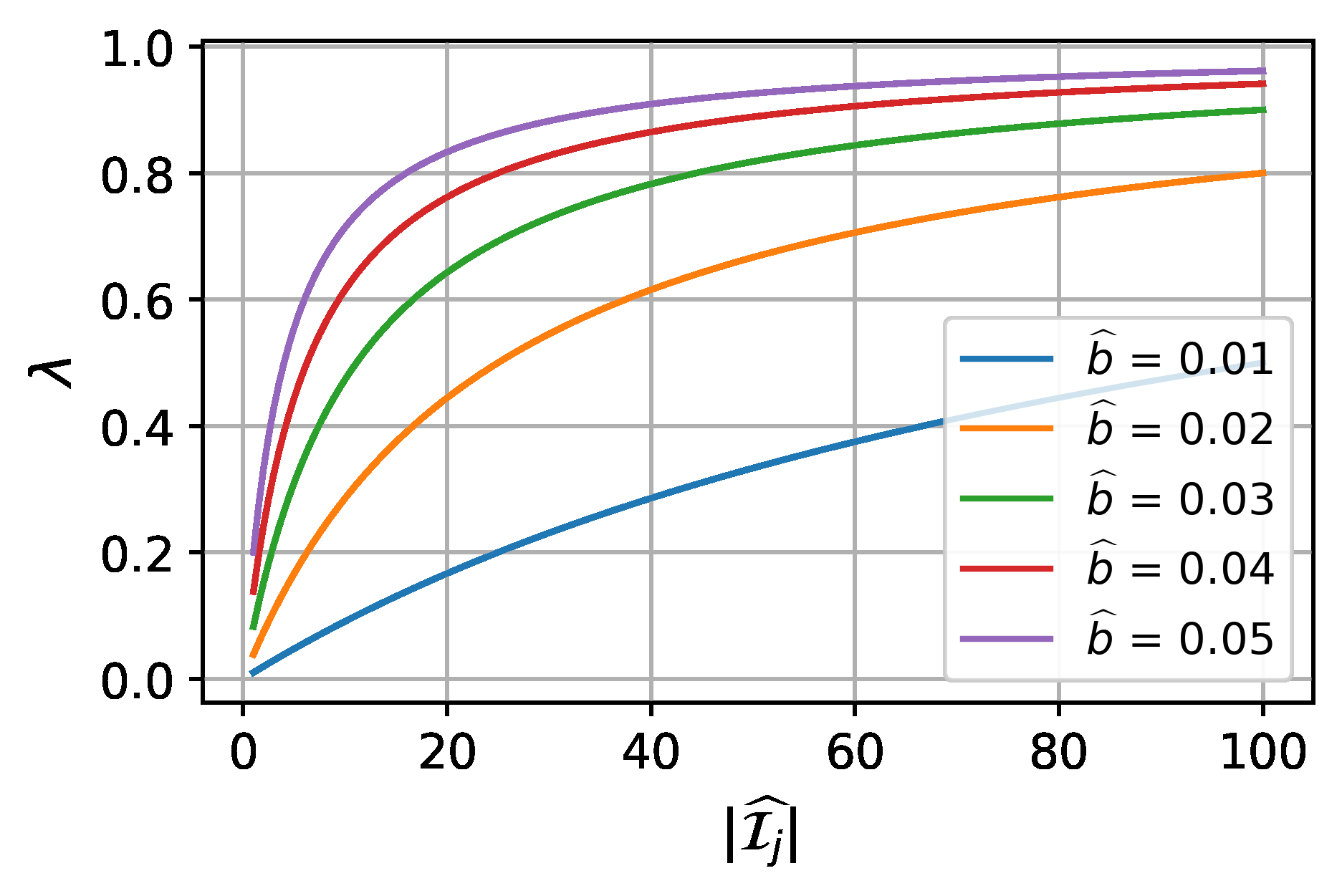
for two constants ˆσ2 and ˆb2. The first constant, ˆσ2, is obtained by computing the average sample variance of Yil, i ∈ I j, across LLMs in the training set. The second constant, ˆb2, is obtained by approximating the IRT bias. We (i) split the training set into two subsets of LLMs; (ii) fit an IRT model in the first part using data from all scenarios; (iii) fit the ability parameter for all the LLMs in the second part using half of the examples of all scenarios; (iv) use that IRT model to predict the correctness (using predicted probabilities) of the unseen examples of scenario j for the models in the second split; (v) average predictions and actual correctness within models, obtaining predicted/actual scenarios scores; (vi) compute their absolute differences, obtaining individual error estimates for models; (vii) average between models, obtaining a final bias estimate, and then square the final number. To give some intuition on how λ is assigned, Figure 2 depicts λ as a function of ˆb and |Îj| when ˆσ2 =.01. From that figure, we see that if the IRT model bias is small, more weight will be given to p-IRT. The curves are steeper when |Îj| is small because the variance of the first estimator decreases faster when |Îj| is small. When the first estimator is obtained by a method that implies an estimator with smaller variance, e.g., anchor points, we apply the same formula but divide ˆσ2 by a constant > 1. By default, we divide ˆσ2 by 4 which is equivalent to halving the standard deviation of the first estimator.
我们基于 Song (1988) 推论 2 导出的启发式选取 $\lambda$。它告诉我们:任意两个估计器 $\hat T_1$ 与 $\hat T_2$(当权重之和为 1 时)的最优线性组合,取决于两估计器的偏差、方差与协方差。若第一个估计器无偏、第二个的方差为零,可以证明最优估计器为 $\lambda \hat T_1 + (1-\lambda) \hat T_2$,其中 $\lambda = b_2^2/(b_2^2 + v_1)$,$b_2$ 表示 $\hat T_2$ 的偏差,$v_1$ 表示 $\hat T_1$ 的方差。为应用该结果,我们假设可能妨碍 gp-IRT 成为好估计器的主要因素是第一个估计器的方差与第二个估计器的偏差,从而把第一个估计器的偏差与第二个估计器的方差近似为零。当第一个估计器来自随机抽样时,我们取
其中 $\hat\sigma^2$ 与 $\hat b^2$ 为两个常数。第一个常数 $\hat\sigma^2$ 由计算训练集各 LLM 在 $Y_{il}$($i \in I_j$)上的平均样本方差得到。第二个常数 $\hat b^2$ 由近似 IRT 偏差得到,步骤为:(i) 把训练集分成两个 LLM 子集;(ii) 用全部场景的数据在第一部分上拟合 IRT 模型;(iii) 用所有场景的一半示例为第二部分的全部 LLM 拟合能力参数;(iv) 用该 IRT 模型(以预测概率)预测第二折模型在场景 $j$ 未观测示例上的正确性;(v) 在各模型内部对预测与实际正确性取平均,得到预测/实际的场景得分;(vi) 计算二者的绝对差,得到各模型的个体误差估计;(vii) 在模型间取平均得到最终偏差估计,再对最终数值取平方。为直观展示 $\lambda$ 如何分配,图 2 描绘了 $\hat\sigma^2 = 0.01$ 时 $\lambda$ 随 $\hat b$ 与 $|\hat I_j|$ 变化的曲线。从该图可见:若 IRT 模型偏差小,给 p-IRT 的权重就更大;曲线在 $|\hat I_j|$ 小时更陡,因为第一个估计器的方差在 $|\hat I_j|$ 小时下降得更快。当第一个估计器来自隐含方差更小的方法(如锚点)时,我们套用同一公式,但把 $\hat\sigma^2$ 除以一个大于 1 的常数。默认地,我们把 $\hat\sigma^2$ 除以 4,等价于把第一个估计器的标准差减半。
[图 2: Understanding the effect of IRT bias and sample size |Îj| in the gp-IRT construction: both quantities are positively related to the weight we give to the raw data in performance estimation.]
图 2:理解 IRT 偏差与样本量 $|\hat I_j|$ 在 gp-IRT 构造中的作用:这两个量都与我们在性能估计中给原始数据的权重正相关。图中曲线为不同 $\hat b$ 下 $\lambda$ 随 $|\hat I_j|$ 的变化($\hat\sigma^2 = 0.01$)——$\hat b$ 越小(IRT 偏差越小),$\lambda$ 越小,即给 p-IRT 的权重越大;$|\hat I_j|$ 小时曲线更陡。
4.3 当 Yil 非二值时使用 IRT(Using IRT when Yil is not binary)
There are situations in which Yil /∈ {0, 1} but Yil ∈ [0, 1]. For example, in AlpacaEval 2.0, the response variable is bounded and can be translated to the interval [0, 1]. Also, some scenarios of HELM and the Open LLM Leaderboard have scores in [0, 1]. We propose a simple and effective fix. The idea behind our method is to binarize Yil by defining a second variable ˜Yil = 1[Yil≥c], for a scenario-dependent constant c. More concretely, for each scenario j, we choose c such that
Σi∈Ij,l∈Ltr Yil ≈ Σi∈Ij,l∈Ltr 1[Yil≥c].
In that way, approximating the average of ˜Yil and Yil should be more or less equivalent. Given that ˜Yil ∈ {0, 1}, we can use the standard IRT tools to model it.
有些情形下 $Y_{il} \notin \{0,1\}$ 但 $Y_{il} \in [0,1]$。例如,在 AlpacaEval 2.0 中,响应变量有界且可变换到区间 $[0,1]$;HELM 与 Open LLM Leaderboard 的一些场景的得分也在 $[0,1]$ 内。我们提出一个简单而有效的修复。方法的想法是:定义第二个变量 $\tilde Y_{il} = \mathbb{1}[Y_{il} \ge c]$($c$ 为随场景而定的常数),把 $Y_{il}$ 二值化(binarize)。更具体地,对每个场景 $j$,我们选择 $c$ 使
这样,$\tilde Y_{il}$ 与 $Y_{il}$ 各自的平均值应大致等价。由于 $\tilde Y_{il} \in \{0, 1\}$,我们可以用标准 IRT 工具为其建模。
4.4 拟合 IRT 模型(Fitting the IRT model)
For the estimation procedure, we resort to variational inference. In particular, we assume that θl ∼ N(µθ1d, 1/uθId), αi ∼ N(µα1d, 1/uαId), and βi ∼ N(µβ, 1/uβ). To take advantage of software for fitting hierarchical Bayesian models (Lalor & Rodriguez, 2023), we introduce (hyper)priors for the prior parameters µθ ∼ N(0, 10), uθ ∼ Γ(1, 1), µα ∼ N(0, 10), uα ∼ Γ(1, 1), µβ ∼ N(0, 10), and uβ ∼ Γ(1, 1). Finally, to obtain point estimates for the model and example-specific parameters θl, αi, and βi, we use the means of their variational distributions. To select the dimension of the IRT model during the fitting procedure, we run a simple validation strategy in the training set and choose the dimension that maximizes the prediction power of the IRT model in the validation split–we consider the dimensions in {2, 5, 10, 15}.
估计流程上,我们借助变分推断(variational inference)。具体地,假设 $\theta_l \sim \mathcal{N}(\mu_\theta \mathbf{1}_d,\; 1/u_\theta\, I_d)$、$\alpha_i \sim \mathcal{N}(\mu_\alpha \mathbf{1}_d,\; 1/u_\alpha\, I_d)$、$\beta_i \sim \mathcal{N}(\mu_\beta,\; 1/u_\beta)$。为利用拟合分层贝叶斯模型的软件(Lalor & Rodriguez, 2023),我们为先验参数引入(超)先验:$\mu_\theta \sim \mathcal{N}(0, 10)$、$u_\theta \sim \Gamma(1, 1)$、$\mu_\alpha \sim \mathcal{N}(0, 10)$、$u_\alpha \sim \Gamma(1, 1)$、$\mu_\beta \sim \mathcal{N}(0, 10)$、$u_\beta \sim \Gamma(1, 1)$。最后,为得到模型特定与示例特定参数 $\theta_l$、$\alpha_i$、$\beta_i$ 的点估计,我们取其变分分布的均值。为在拟合过程中选择 IRT 模型的维度,我们在训练集上运行一个简单的验证策略,选取在验证 split 上预测力最强的维度——我们在 $\{2, 5, 10, 15\}$ 中考虑维度。
5 评测策略的评估(Assessing evaluation strategies)
We assess the ability of the considered evaluation strategies to estimate the performance of LLMs on four popular benchmarks. For a given LLM and a benchmark, each evaluation strategy estimates the performance using evaluation results of this LLM on a given number of examples. We then compare this estimate to the true value, i.e., the performance of this LLM on the complete benchmark.
我们评估所考虑的各评测策略在四个流行基准上估计 LLM 性能的能力。对给定 LLM 与基准,每个评测策略用该 LLM 在给定数量示例上的评测结果来估计其性能;然后我们把该估计与真实值——即该 LLM 在完整基准上的性能——进行比较。
Evaluation pipeline For each benchmark, we first collect publicly available correctness data (Yil's) for a set of LLMs L that have been previously evaluated on this benchmark. Recall that the benchmark is a set of examples I consisting of J disjoint scenarios examples Ij such that I = ∪j∈[J] Ij. We use correctness data corresponding to a subset of LLMs Ltr, i.e., Dtr = {Yil}l∈Ltr,i∈I to (i) find anchor points Îj for each one of the scenarios j ∈ [J] as described in Section 3 and (ii) to obtain estimates for the IRT parameters {(αi,βi)}i∈I as described in Section 4. We call this "train" set of models as their correctness data is used to identify anchor points and fit the parameters associated with our evaluation strategies. The remaining set of "test" models Lte is used to quantify the error of our evaluation strategies in practice. For each LLM in the test set, l ∈ Lte, we observe its correctness on the anchor points, i.e., {Yil}i∈Îj, and use it to obtain benchmark performance estimates as described in Sections 3 and 4. The estimate is then compared to the ground truth, i.e., performance of this LLM on the entirety of the benchmark.
评测流水线。对每个基准,我们首先收集曾在该基准上被完整评测过的一组 LLM $\mathcal{L}$ 的公开正确性数据($Y_{il}$)。回顾:基准是由 $J$ 个互斥场景的示例 $I_j$ 组成的示例集 $I$,即 $I = \bigcup_{j\in[J]} I_j$。我们把对应于 LLM 子集 $\mathcal{L}_{tr}$ 的正确性数据,即 $\mathcal{D}_{tr} = \{Y_{il}\}_{l\in\mathcal{L}_{tr},\, i\in I}$,用于:(i) 按第 3 节所述为每个场景 $j \in [J]$ 找锚点 $\hat I_j$;(ii) 按第 4 节所述得到 IRT 参数 $\{(\alpha_i, \beta_i)\}_{i\in I}$ 的估计。我们称这组模型为「训练」集,因为其正确性数据被用于识别锚点并拟合与评测策略相关的参数。其余的「测试」模型集 $\mathcal{L}_{te}$ 用于量化我们的评测策略在实践中的误差。对测试集中每个 LLM $l \in \mathcal{L}_{te}$,我们观察其在锚点上的正确性 $\{Y_{il}\}_{i\in\hat I_j}$,并按第 3、4 节所述用它得到基准性能估计;再将该估计与真值——该 LLM 在整个基准上的性能——比较。
We consider two train-test model split scenarios: (i) random split and (ii) by date, i.e., using the most recent models for testing. The latter split better represents practical use cases, while also being more challenging as it is likely to result in a distribution shift between the train and test models due to improving model capabilities over time that might affect the effectiveness of anchor points and the IRT model.
我们考虑两种训练-测试模型划分:(i) 随机划分;(ii) 按日期划分,即用最新模型做测试。后一种更贴近实际用例,同时也更难:模型能力随时间提升,很可能造成训练/测试模型间的分布偏移,可能影响锚点与 IRT 模型的有效性。
Benchmarks and models We describe the size and composition of the four benchmarks, as well as the corresponding LLMs (see Appendix D for additional details):
基准与模型。我们描述四个基准的规模与构成,以及相应的 LLM(更多细节见附录 D):
HuggingFace's Open LLM Leaderboard (Beeching et al., 2023) consists of 6 scenarios, approx. 29K examples in total. Performance on each of the scenarios is measured with accuracy and the overall benchmark performance is equal to the average of scenario accuracies. We collect evaluation results for 395 LLMs from the Leaderboard's website and use 75% for training and 25% for testing (split either randomly or by date as described above).
- HuggingFace 的 Open LLM Leaderboard(Beeching et al., 2023)由 6 个场景组成,总计约 29K 个示例。各场景的性能以准确率度量,基准整体性能等于各场景准确率的平均。我们从 Leaderboard 网站收集了 395 个 LLM 的评测结果,75% 用于训练、25% 用于测试(按上述方式随机或按日期划分)。
MMLU (Hendrycks et al., 2020) is a multiple choice QA scenario consisting of 57 subjects (subscenarios) comprising approx. 14K examples. Performance on MMLU is measured by averaging the accuracies on each of the categories. MMLU is one of the 6 scenarios of the Open LLM Leaderboard and we consider the same set of 395 LLMs and train-test splits. The reason to consider it separately is its immense popularity when comparing LLMs (Touvron et al., 2023; Achiam et al., 2023; Team et al., 2023) and inclusion into several other benchmarks.
- MMLU(Hendrycks et al., 2020)是一个选择题问答场景,由 57 个学科(子场景)组成,共约 14K 个示例。MMLU 的性能由各类别准确率的平均度量。MMLU 是 Open LLM Leaderboard 的 6 个场景之一,我们考虑同样的 395 个 LLM 集合与训练-测试划分。单独考察它的原因是:它在比较 LLM 时极为流行(Touvron et al., 2023; Achiam et al., 2023; Team et al., 2023),并被纳入多个其他基准。
For HELM (Liang et al., 2022), we use HELM Lite v1.0.0, which has the 10 core scenarios (total of approx. 10K evaluation examples) and 30 models that have their performances registered for all scenarios. Performance metrics for each scenario vary and can be non-binary (e.g., F1 score), and the overall performance on the benchmark is measured with mean win rate across scenarios. For this benchmark, the dates models were added are not available. Instead, we split models based on the organizations that trained them to create more challenging train-test splits, e.g., all OpenAI models are either in train or in test. For the random train-test split we use 11-fold cross-validation. That is, we partition the set of all LLMs into k = 11 parts and, for each one of these parts, we use one of them to test and k − 1 parts for training. Then, we average the results over the choice of the testing part.
- 对 HELM(Liang et al., 2022),我们使用 HELM Lite v1.0.0:它有 10 个核心场景(总计约 10K 个评测示例)以及在所有场景上均有性能记录的 30 个模型。各场景的性能指标不一,且可以是非二值的(如 F1 分数);基准整体性能以跨场景的平均胜率度量。对这个基准,模型加入的日期不可得。作为替代,我们按训练模型的组织来划分,以制造更有挑战的训练-测试划分,例如所有 OpenAI 模型要么全在训练集、要么全在测试集。随机训练-测试划分则用 11 折交叉验证:把全部 LLM 集合分成 $k = 11$ 份,对每一份,用其中一份做测试、其余 $k-1$ 份做训练,再对不同测试份的选择取平均。
AlpacaEval 2.0 (Li et al., 2023) consists of 100 LLMs evaluated on 805 examples. Although it is a fairly small benchmark, evaluation is expensive as it requires GPT-4 as a judge. For each input, GPT-4 compares the responses of a candidate LLM and a baseline LLM (currently also GPT-4) and declares a winner. The average win rate is used to measure the overall performance. When splitting the data by date, we pick 25% most recent models for testing and the rest for training. For the random split, we employ 4-fold cross-validation analogous to HELM.
- AlpacaEval 2.0(Li et al., 2023)由在 805 个示例上被评测的 100 个 LLM 组成。虽然它是相当小的基准,评测却很昂贵,因为它需要 GPT-4 做裁判:对每个输入,GPT-4 比较候选 LLM 与基线 LLM(目前也是 GPT-4)的回答并宣布胜者;平均胜率用于度量整体性能(原文脚注 4:实验中考察的 AlpacaEval 2.0 使用连续偏好而非二值)。按日期划分时,我们取最近的 25% 模型做测试、其余做训练;随机划分则用与 HELM 类似的 4 折交叉验证。
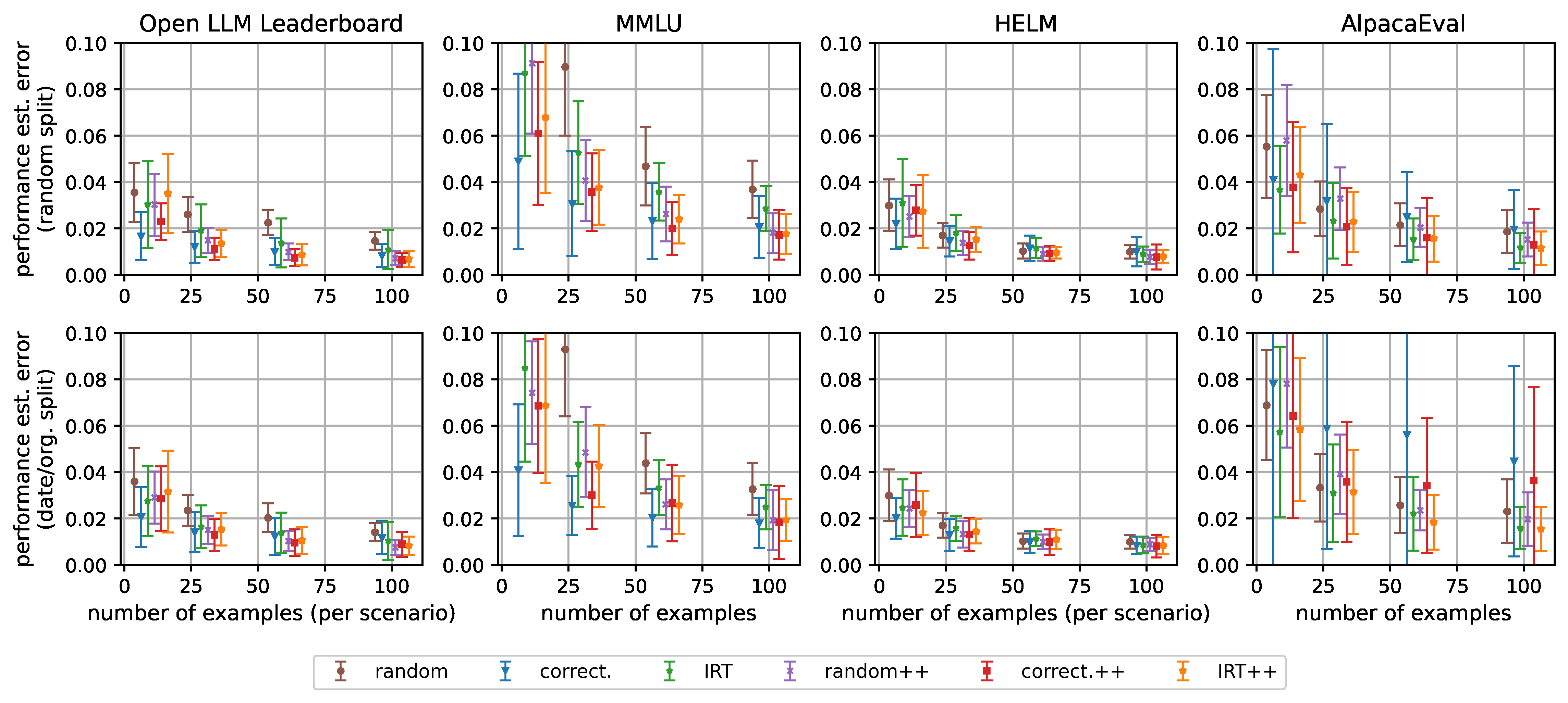
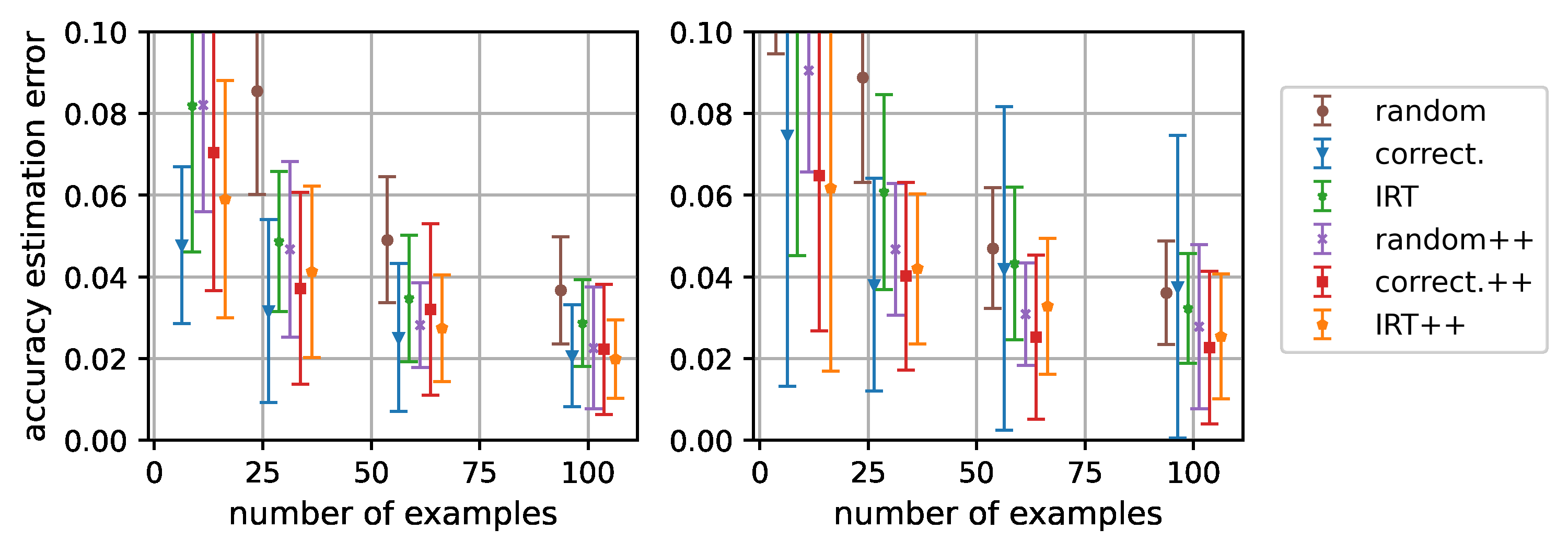
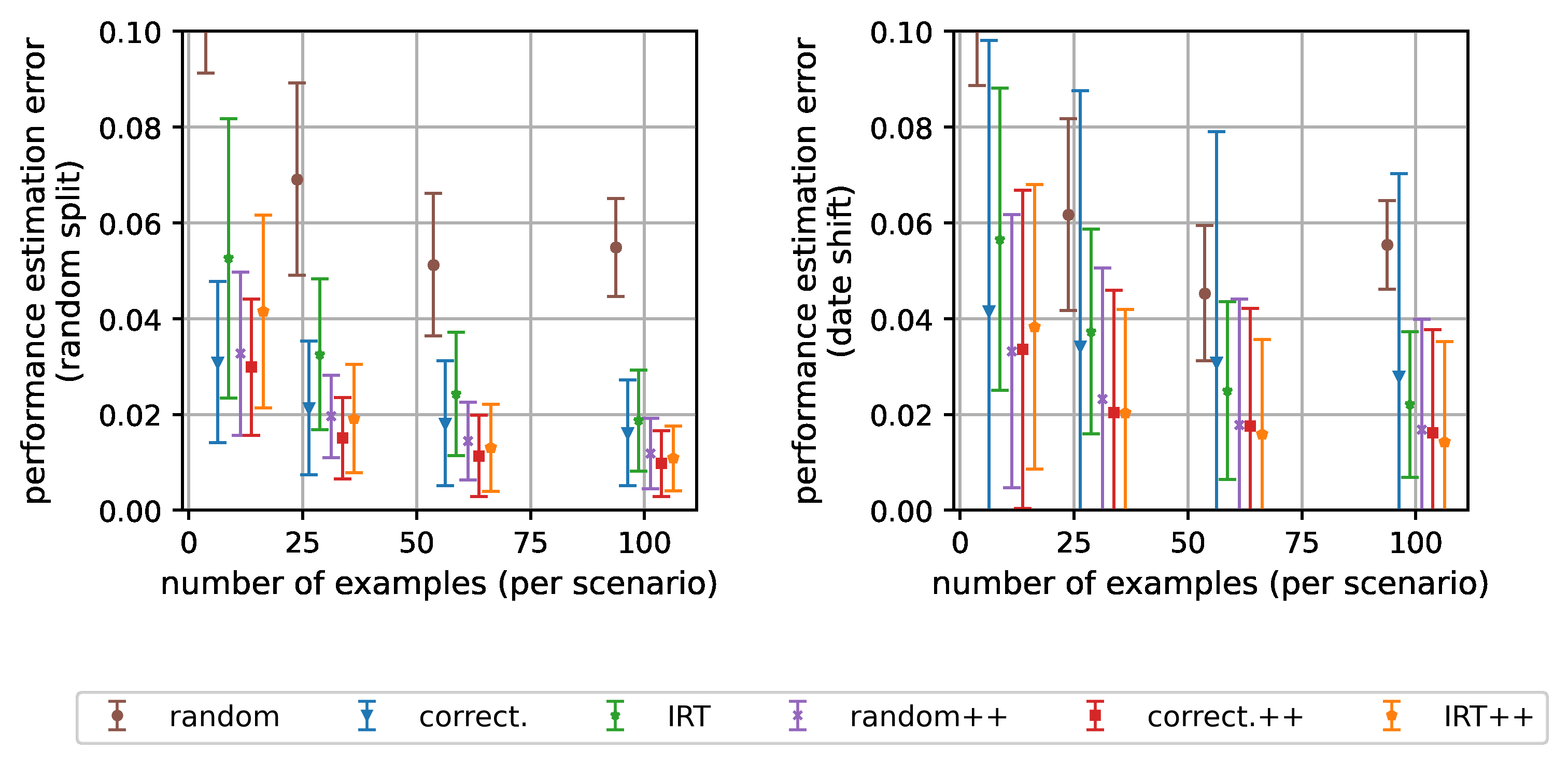
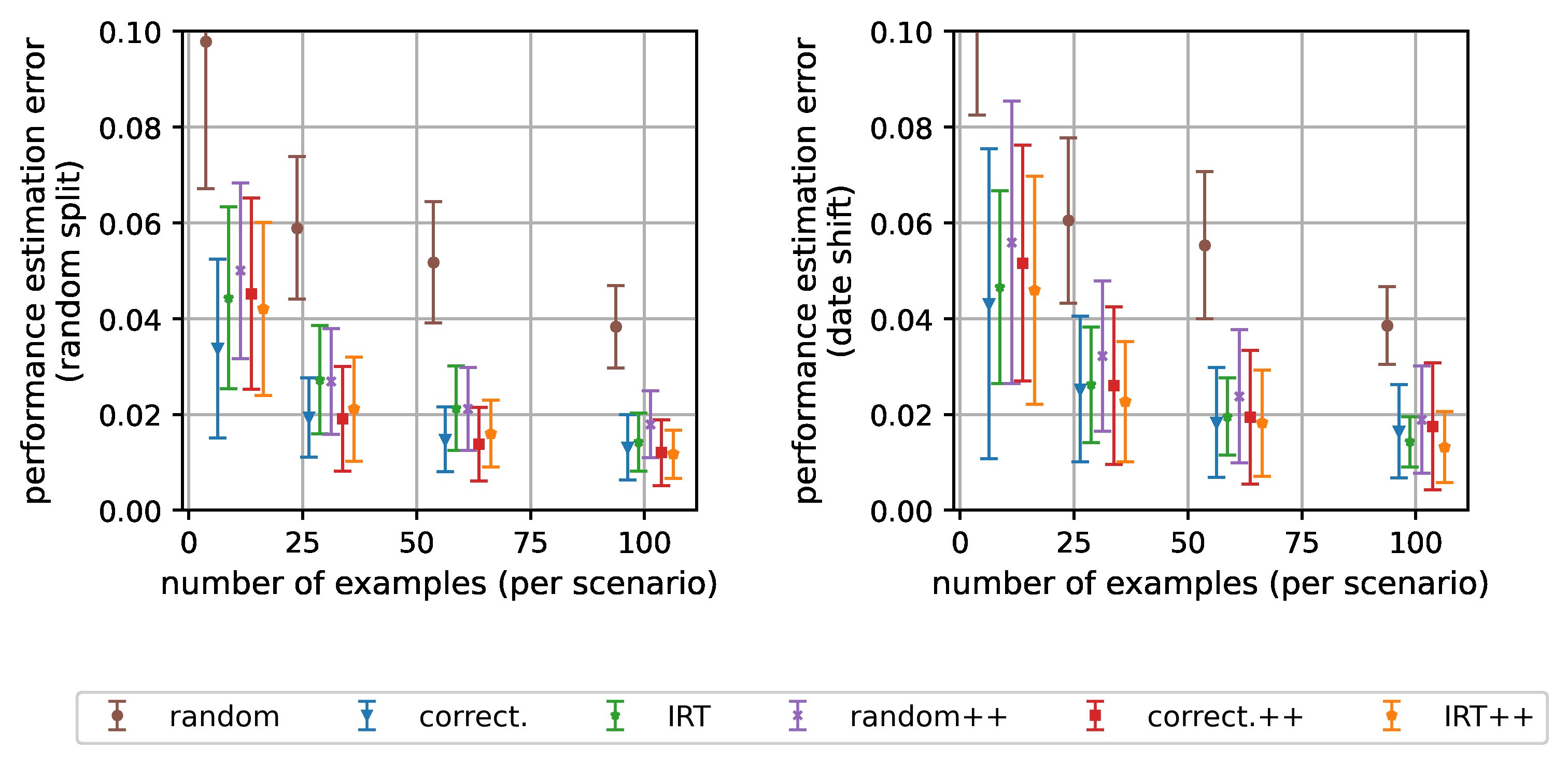
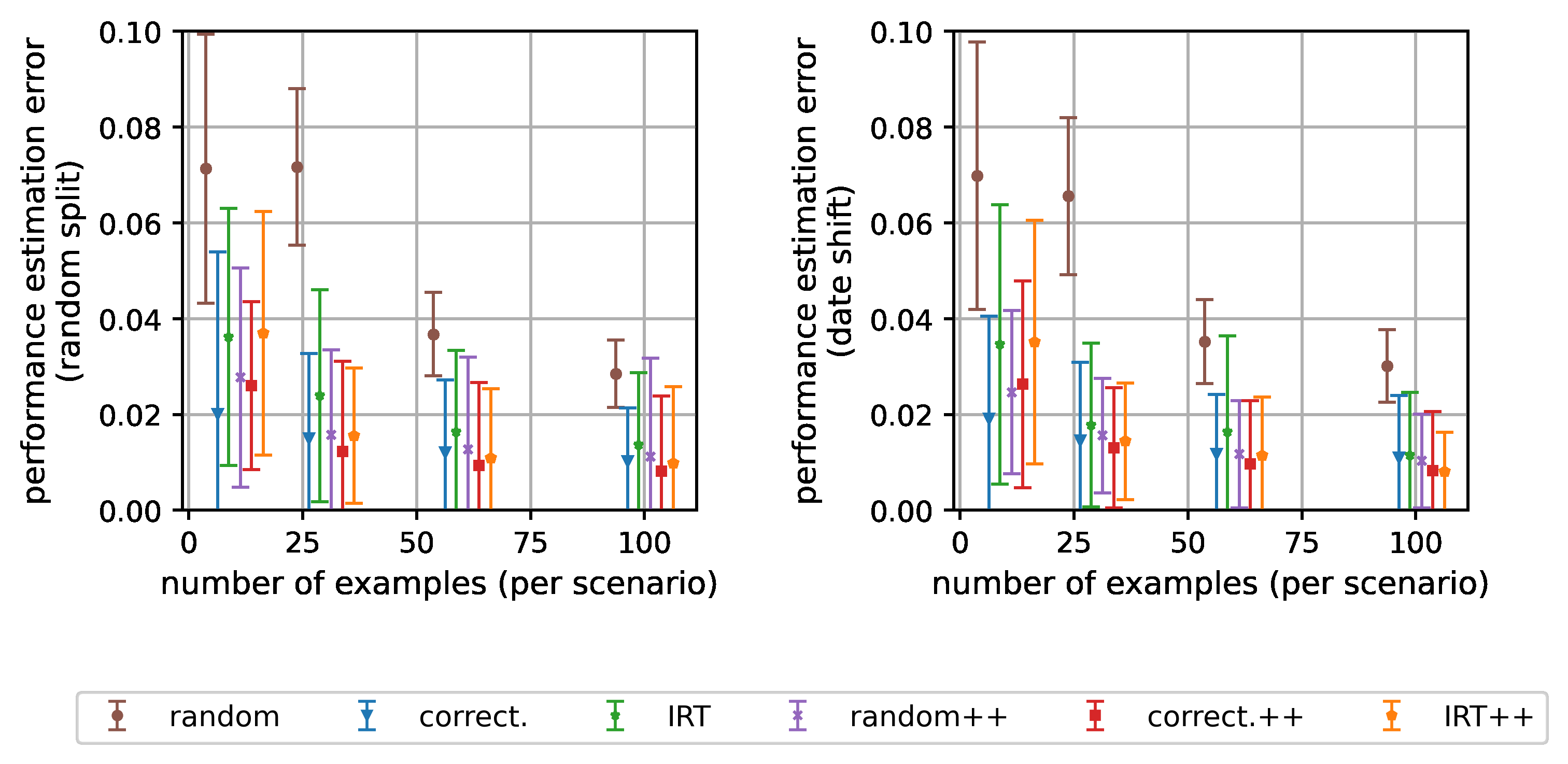
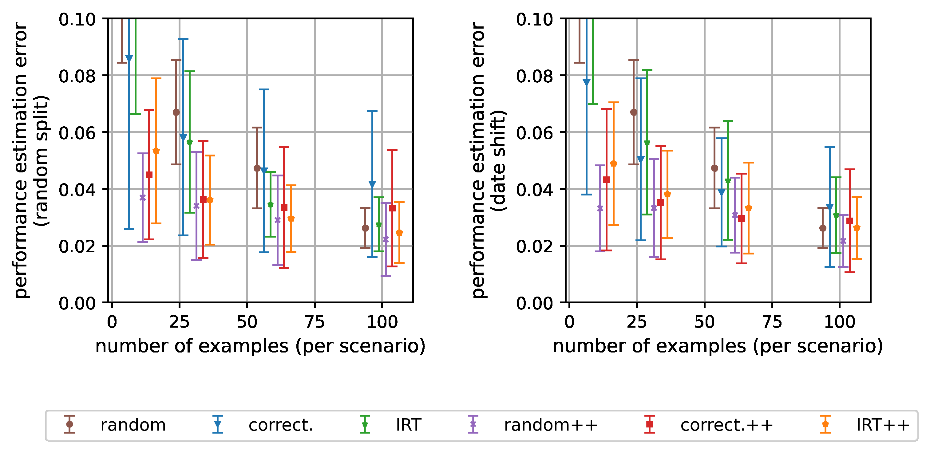
[图 3: Performance estimation error per benchmark (columns) tested on random (top row) and recent (bottom row) LLMs for increasing number of evaluation examples. 100 examples per scenario is sufficient to achieve ≈2% average performance estimation error across benchmarks and evaluated LLMs. This corresponds to 600 out of 29K examples for Open LLM Leaderboard, 100 out of 14K examples for MMLU, 1000 out of 10K examples for HELM, and 100 out of 800 examples for AlpacaEval 2.0.]
图 3:各基准(列)分别在随机 LLM(上排)与最新 LLM(下排)上测试时,性能估计误差随评测示例数的增加而下降。每场景 100 个示例即可在所有基准与被评 LLM 上达到约 2% 的平均性能估计误差——这相当于 Open LLM Leaderboard 从 29K 例中取 600 例、MMLU 从 14K 例中取 100 例、HELM 从 10K 例中取 1000 例、AlpacaEval 2.0 从约 800 例中取 100 例。
Evaluation strategies We consider 3 strategies presented in §3 for selecting a subset of examples for efficient evaluation: "random" for stratified random sampling, "correctness" for clustering correctness of models in the train set, and "IRT" for clustering the example representations obtained from the IRT model fit on the train set. For each strategy, we evaluate the vanilla variation, i.e., simply using the performance of a test LLM on the (weighted) set of selected examples to estimate its performance on the full benchmark, and "++" variation that adjusts this estimate using the IRT model as described in equation (4.4). In total, we assess six evaluation strategies. Results are averaged over 5 restarts.
评测策略。我们考虑 §3 提出的 3 种为高效评测选择示例子集的策略:「random」即分层随机抽样;「correctness」即对训练集模型的正确性聚类;「IRT」即对在训练集上拟合的 IRT 模型所得示例表示聚类。对每种策略,我们评估两个变体:朴素(vanilla)变体,即直接用测试 LLM 在所选(加权)示例集上的性能来估计其在完整基准上的性能;「++」变体,即按式 4.4 用 IRT 模型校正该估计。总计我们评估六种评测策略。结果为 5 次重启的平均。
Key findings We investigate the effectiveness of strategies as we increase the number of examples available for evaluating test LLMs. Results for both train-test split scenarios are presented in Figure 3 (see also Figure 14 for Spearman's rank correlations). Our main conclusions are:
Our approach to reducing evaluation costs is effective. The best-performing strategies achieve estimation error within 2% on all benchmarks with 100 examples or less per dataset or scenario. For example, for MMLU this reduces the evaluation cost by a factor of 140 (from 14k to 100). For Open LLM Leaderboard even 30 examples per scenario is enough, reducing the evaluation cost by a factor of 160 (from 29K to 180).
Most strategies perform well when there is a temporal shift between the train and test LLM's (see the lower row of plots in Figure 3 for the results with "by date" split). Thus our approaches for reducing evaluation costs remain practical when evaluating the performance of newer, more capable LLMs and can help save GPU hours when evaluating future LLMs and/or checkpoints during pre-training.
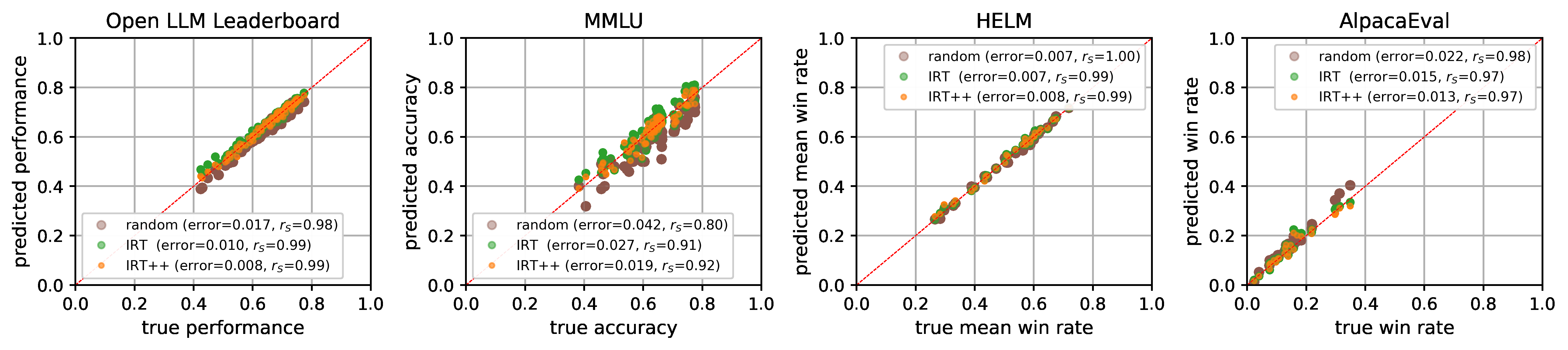
IRT-based methods ("IRT" and "IRT++") perform consistently well across benchmarks and train-test splits. The gp-IRT ("++") variation always improves or matches its vanilla counterpart, while adding only a few seconds to the evaluation time (see Figure 13). Thus we use the IRT-based anchor examples to construct tiny versions (100 examples per scenario) of each of the benchmarks and release them along with the gp-IRT tool (code and pre-trained IRT model) for efficient evaluation of future LLMs. We present additional evaluations of tinyBenchmarks in Figure 4 for one of the 5 random seeds in which the random sampling underperforms. In Appendix B, we conduct an exploratory analysis of the examples comprising tinyMMLU.
关键发现。我们研究当可用于评测测试 LLM 的示例数增加时,各策略效果如何变化。两种训练-测试划分的结果见图 3(Spearman 秩相关见图 14)。我们的主要结论:
- 我们降低评测成本的做法是有效的。表现最好的策略以每数据集或每场景 100 个或更少的示例,在所有基准上把估计误差控制在 2% 以内。例如对 MMLU,这把评测成本降低了 140 倍(14K → 100);对 Open LLM Leaderboard,每场景 30 个示例就够,评测成本降低 160 倍(29K → 180)。
- 当训练与测试 LLM 之间存在时间偏移时,多数策略仍表现良好(「按日期」划分的结果见图 3 下排)。因此,在评测更新、更强的 LLM 时,我们降低评测成本的做法依然实用,可在评测未来 LLM 与/或预训练期间的检查点时节省 GPU 时。
- 基于 IRT 的方法(「IRT」与「IRT++」)在各基准与各训练-测试划分下都持续表现良好。gp-IRT(「++」)变体总是优于或持平其朴素对应,而只给评测时间增加几秒(见图 13)。因此,我们用基于 IRT 的锚点示例构建每个基准的 tiny 版本(每场景 100 例),并连同 gp-IRT 工具(代码与预训练 IRT 模型)一起发布,用于未来 LLM 的高效评测。图 4 展示了 5 个随机种子中随机抽样表现欠佳的那个种子下 tinyBenchmarks 的额外评测。附录 B 对构成 tinyMMLU 的示例做了探索性分析。
[图 4: Predicted performance compared with true performance for the four benchmarks (columns) and recent LLMs. We verify the efficacy of the evaluation strategies (IRT and IRT++) we chose to construct tinyBenchmarks.]
图 4:四个基准(列)在最新 LLM 上的预测性能与真实性能对比。我们借此验证为构建 tinyBenchmarks 所选评测策略(IRT 与 IRT++)的效力。
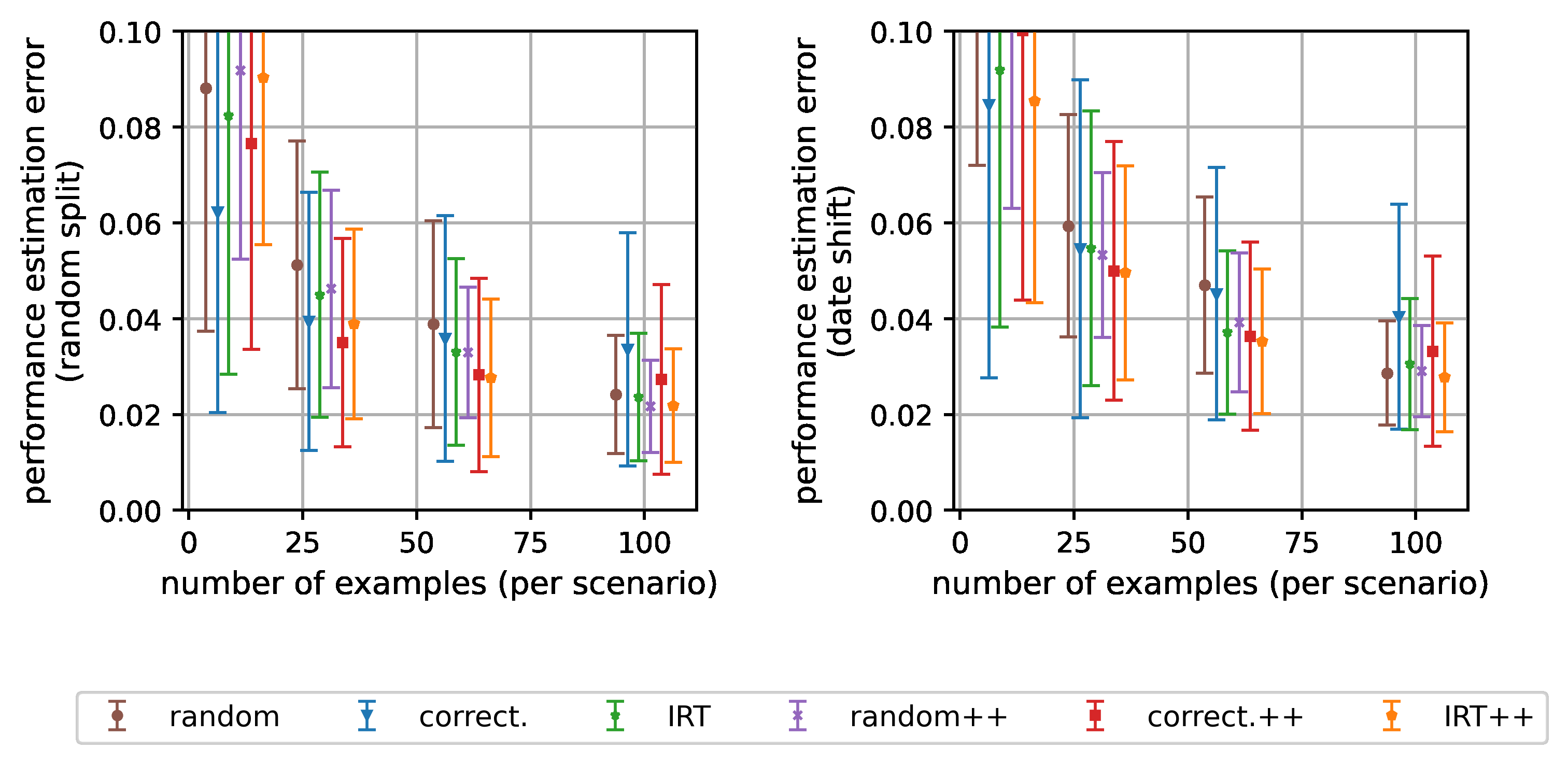
Specialized LLMs In our previous experiments the test set of LLMs consisted of either a random subset of models or the most recent ones. Both of these test sets are dominated by base and instruction-tuned LLMs. Here we assess the ability of the considered strategies to predict the performance of specialized LLMs, i.e., models fine-tuned for specific domains such as code, biology, or finance. We consider MMLU benchmark and collect a new hand-picked test set of 40 specialized models. Such models are likely to have unique strengths and perform well in specific MMLU categories while relatively underperforming on others. Thus, their correctness patterns might be different from those in the train set, posing a challenge for our evaluation strategies. We present results in Figure 5. As we anticipated, the correctness-based anchor strategy deteriorates when tested on specialized LLMs. In contrast to the IRT-based anchors that are only slightly affected, demonstrating their robustness and supporting our choice to use them for tinyBenchmarks construction.
领域特化 LLM。此前实验中,LLM 测试集由随机抽取的模型或最新模型组成,两类测试集都以基座(base)与指令微调(instruction-tuned)的 LLM 为主。这里我们评估所考虑策略预测领域特化(specialized)LLM——即为代码、生物、金融等特定领域微调的模型——性能的能力。我们考虑 MMLU 基准,并收集了一个手工挑选的 40 个特化模型组成的新测试集。这类模型很可能有独特强项:在特定 MMLU 类别上表现好,而在其他类别上相对弱。因此,它们的正确性模式可能与训练集中的不同,对我们的评测策略构成挑战。结果见图 5。正如预期,基于正确性的锚点策略在特化 LLM 上测试时显著退化;相比之下,基于 IRT 的锚点只受到轻微影响,展示了其鲁棒性,也支持了我们用它们构建 tinyBenchmarks 的选择。
[图 5: Estimation error on specialized LLMs (right) compared to error on random LLMs (left) on MMLU. Correctness-based example selection is affected the most by this distribution shift.]
图 5:MMLU 上特化 LLM 的估计误差(右)与随机 LLM 的估计误差(左)对比。基于正确性的示例选择受这种分布偏移的影响最大。
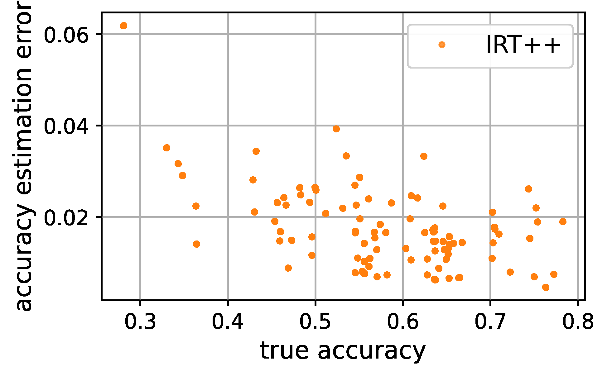
Estimation error analysis We present a more detailed view of the estimation error of the best performing "IRT++" evaluation strategy on MMLU with 100 examples. In Figure 6 we plot estimation error against the actual accuracy of 99 test LLMs for a random train-test split. Our strategy can estimate the performance of more capable LLMs slightly better, although there is no strong dependency. We also note that the estimation error never exceeds 4% (except for one LLM with extremely low performance). Recall that the average error is 2% as shown in Figure 3, supporting the reliability of our evaluation approach.
估计误差分析。我们更细致地查看表现最好的「IRT++」评测策略在 MMLU、100 示例下的估计误差。图 6 画出随机训练-测试划分下 99 个测试 LLM 的估计误差对其真实准确率的散点。我们的策略对能力更强 LLM 的估计略好,尽管依赖并不强。我们还注意到,估计误差从不超过 4%(仅一个性能极低的 LLM 例外)。回顾图 3 所示平均误差为 2%,支持了我们评测方法的可靠性。
[图 6: Spread of estimation errors across a random subset of LLMs with varying capabilities on MMLU. The error tends to be slightly lower for more capable models. The worst case error across almost all models is ≤ 4%.]
图 6:MMLU 上能力各异的随机 LLM 子集的估计误差分布。误差对能力更强的模型往往略低;几乎所有模型的最坏情形误差 ≤ 4%。
6 结论(Conclusion)
In this paper, we demonstrate it is possible to accurately assess the capabilities of LLMs with a fraction (sometimes two orders of magnitude smaller) of the examples in common benchmark datasets by leveraging models of educational assessments from psychometrics. This leads directly to savings in terms of the monetary costs associated with evaluating LLMs, but also the computational and environmental costs. For practitioners, the computational cost savings are especially convenient because they enable them to evaluate LLMs more frequently during fine-tuning and prompt engineering.
本文证明:借助心理测量学中来自教育测评的模型,用常见基准数据集的一小部分(有时小两个数量级)示例即可准确评估 LLM 的能力。这直接节省了评测 LLM 的财务成本,以及算力与环境成本。对从业者而言,算力成本的节省尤其便利,因为它使他们能在微调与提示工程期间更频繁地评测 LLM。
Based on our results we are releasing tinyBenchmarks, pre-selected subsets of examples from the widely adopted LLM benchmarks. tinyBenchmarks are simply small datasets that are straightforward to use to evaluate LLMs cheaply. We are also releasing an IRT-based tool to enhance performance estimation. The tool provides code and IRT parameters trained on the corresponding benchmarks and can be run on a CPU in a few seconds.
基于我们的结果,我们发布 tinyBenchmarks——从被广泛采用的 LLM 基准中预先选出的示例子集。tinyBenchmarks 就是小型数据集,可直接用于廉价地评测 LLM。我们还发布一个基于 IRT 的工具以增强性能估计:该工具提供代码与在相应基准上训练好的 IRT 参数,可在 CPU 上数秒内运行。
6.1 扩展(Extensions)
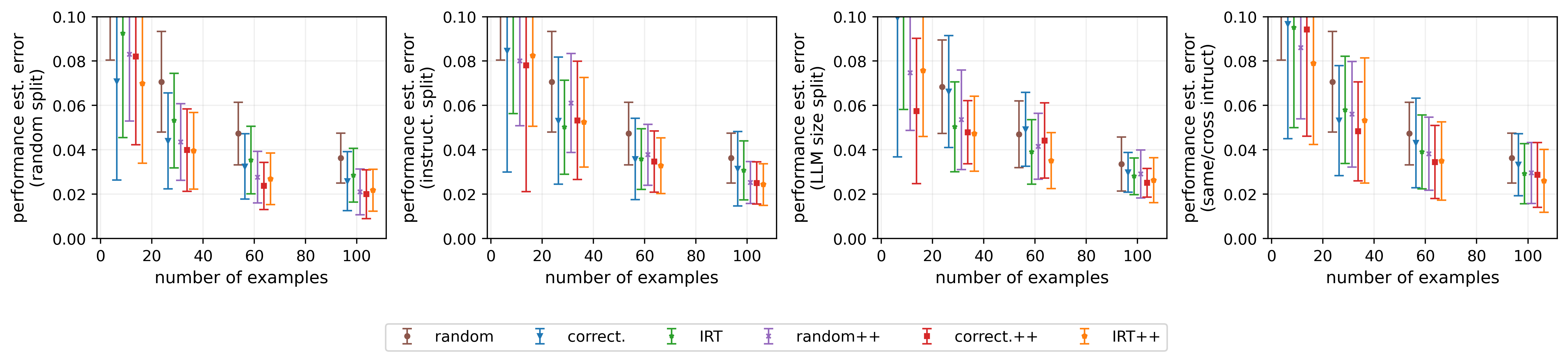
Prompt evaluation A persistent challenge in prompt-based model evaluation is the influence the prompting setup has on model predictions (see, e.g., Lu et al., 2022; Mishra et al., 2022; Min et al., 2022; Yoo et al., 2022; Weber et al., 2023b; Wei et al., 2023). We can use the previously described approaches to make predictions across different prompting setups. This way, we can estimate how well a model will do on a new set of prompts using just a few evaluations, or how a new model will perform on a given prompt. To test this idea, we train an IRT model on the prediction data from Weber et al. (2023a), containing evaluations of eight LLaMA LLMs (vanilla or instruction tuned on the Alpaca self-instruct dataset; Touvron et al., 2023; Taori et al., 2023) for the ANLI dataset (Nie et al., 2020). The dataset consists of evaluations of the 750 data points wrapped with 15 different instruction templates sourced from the promptsource collection (P3; Bach et al., 2022). Similarly to our previous experiments, we evaluate random splits and splits featuring distribution shifts (across model sizes and different instruction templates). For model size, we put all models with sizes 7B, 13B, and 30B in the training set while the models with size 65B go to the test set. For splits related to prompts templates, we consider two different approaches: first, we conduct a 2-fold cross-validation rotating instruction templates; second, we consider using the same and different instruction templates in the in-context-learning examples and in the input example alternating the strategies in the training and test sets. Results in Figure 7 suggest that prompt-based model evaluation can be efficiently carried out with the methods introduced in this work, even in the presence of several practical distribution shifts.
提示评测(prompt evaluation)。基于提示的模型评测中一个持续的挑战,是提示设定(prompting setup)对模型预测的影响(见 Lu et al., 2022; Mishra et al., 2022; Min et al., 2022; Yoo et al., 2022; Weber et al., 2023b; Wei et al., 2023)。我们可以用前述方法跨不同提示设定做预测:这样,只需少量评测即可估计一个模型在一组新提示上的表现,或一个新模型在给定提示上的表现。为检验这个想法,我们在 Weber et al. (2023a) 的预测数据上训练一个 IRT 模型;该数据包含 8 个 LLaMA LLM(原始版,或在 Alpaca self-instruct 数据集上指令微调版;Touvron et al., 2023; Taori et al., 2023)在 ANLI 数据集(Nie et al., 2020)上的评测。该数据集由 750 个数据点套上 15 个不同指令模板(取自 promptsource 集合,即 P3;Bach et al., 2022)后的评测组成。与之前的实验类似,我们评估随机划分以及带分布偏移的划分(跨模型规模与跨不同指令模板)。模型规模方面,7B、13B、30B 的模型全部放进训练集,65B 的模型放进测试集。提示模板相关的划分考虑两种做法:其一,做轮换指令模板的 2 折交叉验证;其二,考虑在上下文学习示例与输入示例中使用相同与不同的指令模板,并在训练集与测试集之间交替这些策略。图 7 的结果表明,用本文方法可以高效地进行基于提示的模型评测,即使存在多种实际分布偏移。
[图 7: Estimation error when predicting the performance of prompt templates. The results demonstrate that using our methods for efficient prompt-based model evaluation is a promising application.]
图 7:预测提示模板性能时的估计误差。结果表明,把我们的方法用于高效的基于提示的模型评测是一个有前景的应用。
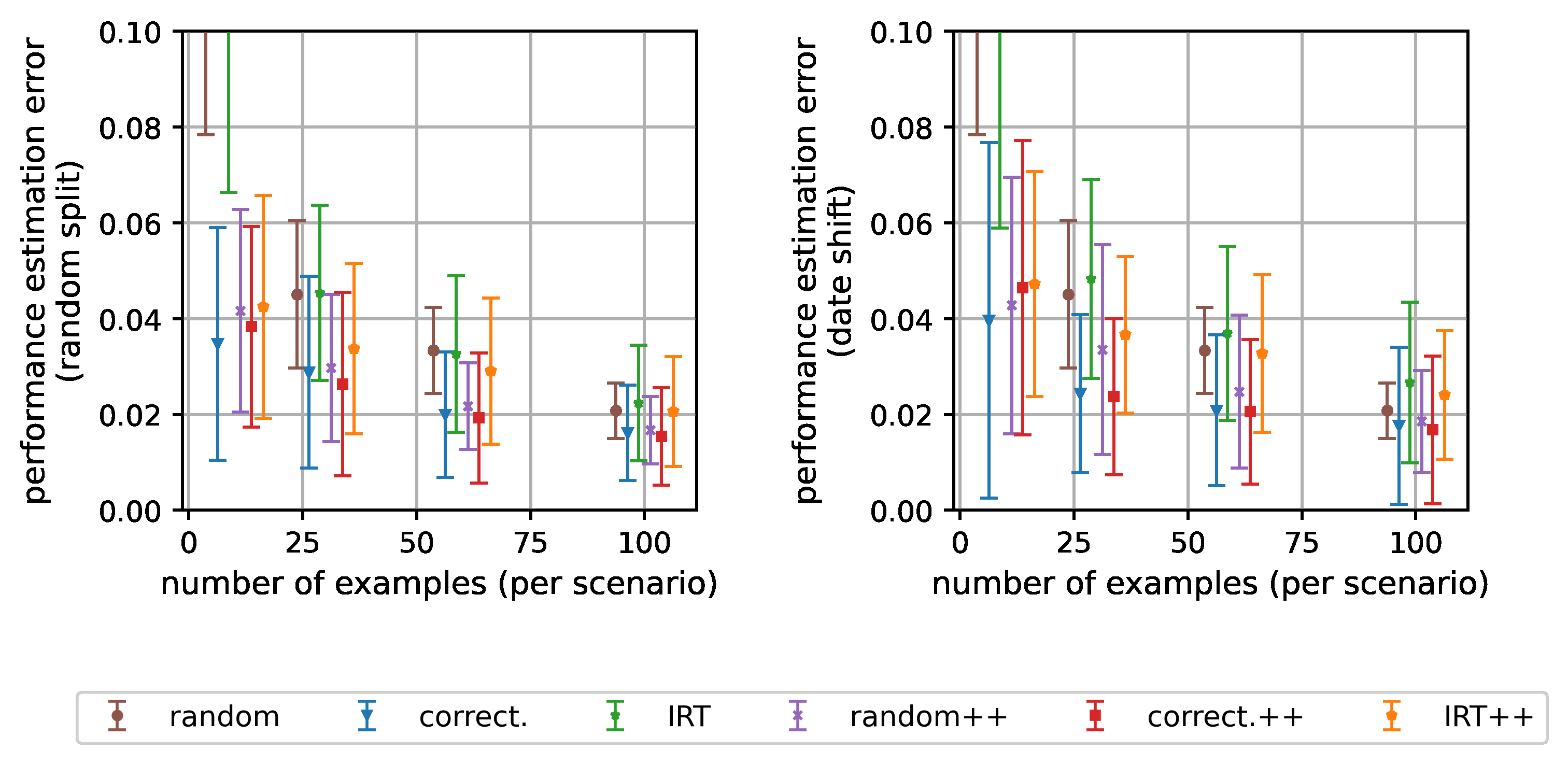
Adaptive testing We expect further performance estimation improvements can be squeezed out by more sophisticated applications of similar ideas. For example, instead of pre-selecting a subset of examples before evaluating the LLM, it may be possible to select the examples adaptively during the evaluation process. This idea is widely used in the computerized-assisted testing algorithms behind many standardized tests. We demonstrate preliminary results on MMLU using an adaptive IRT variant in Figure 8 (see Figure 16 for results on more benchmarks). Although the estimation performance has improved, our current implementation takes over 5 minutes to run, which might not be as appealing practically.
自适应测试(adaptive testing)。我们预计,更精巧地应用类似想法还能进一步榨出性能估计的改进。例如,与其在评测 LLM 之前预先选定一个示例子集,不如在评测过程中自适应地选择示例。这一思想广泛应用于许多标准化考试背后的机考辅助测试算法。图 8 展示了我们在 MMLU 上用自适应 IRT 变体得到的初步结果(更多基准见图 16)。尽管估计性能有所提升,我们当前的实现要跑 5 分钟以上,实用性可能欠佳。
[图 8: Preliminary adaptive testing results on MMLU.]
图 8:MMLU 上的初步自适应测试结果。图中比较 random、IRT、IRT++ 与 adaptIRT++ 四种策略的得分估计误差随已见样本数(20–100)的变化:adaptIRT++ 的误差曲线整体最低。
(译注:原图为折线图,横轴为已见样本数,纵轴为得分估计误差,曲线自上而下大体为 random、IRT、IRT++、adaptIRT++。)
6.2 局限(Limitations)
The main limitations of the methods described in this paper are related to potential severe distribution shifts. Taking MMLU as an example, we anticipate larger performance estimation errors for models that fail on simple questions while answering complicated ones correctly, thus altering the correctness patterns. This might be caused by significant architecture or pre-training data changes. A rapid increase in LLM capabilities may also cause extrapolation errors. To alleviate these problems, we recommend periodically updating the curated examples and IRT parameter estimates using data from more modern LLMs.
本文所述方法的主要局限与潜在的严重分布偏移有关。以 MMLU 为例,我们预计对「简单题答错、而难题反而答对」从而颠覆了正确性模式的模型,性能估计误差会更大。这可能由架构或预训练数据的重大变化引起;LLM 能力的快速跃升也可能造成外推误差。为缓解这些问题,我们建议定期用更现代的 LLM 的数据更新精选示例与 IRT 参数估计。
致谢(Acknowledgements)
We are grateful for the help provided by Yotam Perlitz in downloading data from HELM. This paper is based upon work supported by the National Science Foundation (NSF) under grants no. 2027737 and 2113373.
我们感谢 Yotam Perlitz 在下载 HELM 数据方面提供的帮助。本文基于美国国家科学基金会(NSF)第 2027737 与 2113373 号拨款支持的工作。
影响声明(Impact Statement)
This paper presents work whose goal is to advance the field of Machine Learning. There are many potential societal consequences of our work, none which we feel must be specifically highlighted here.
本文呈现的工作旨在推动机器学习领域的发展。我们的工作可能有许多潜在的社会性后果,但没有哪一条是我们认为必须在此特别指出的。
附录 A 子场景样本数不同时的评测(Evaluation when subscenarios have different number of samples)
Suppose we want to estimate the performance of a scenario j which is composed of sj subscenarios. Denote the set of examples in each subscenario of j as Ijk, for k ∈ {1, ··· , sj}. Then, Ij = ∪kIjk, with disjoint Ijk's. For a given LLM l, our main goal is then to estimate 1/sj Σk 1/|Ijk| Σi∈Ijk Yil. See that we can write
1/sj Σk 1/|Ijk| Σi∈Ijk Yil = Σk Σi∈Ijk 1/(sj|Ijk|) Yil = Σi∈Ij ω¯iYil.
This tells us that we can represent the performance of model l as a weighted average instead of a simple average. In our code, ωi ≜ |Ij|· ω¯i's are called balance weights and ω¯i's are called normalized balance weights. In Section 3, when computing the estimates using the stratified random sampling strategy, the weights for each example are still given by 1/|Îj| (because subscenarios should already be equally represented) but when using the clustering ideas, the weight for each anchor point is given by the sum of ω¯i's of all items in its cluster. We do not apply any weighting when fitting the IRT models but only when computing the p-IRT (and gp-IRT) estimate:
ˆZp-IRT jl = λˆ/|Îj| Σi∈Îj ωiYil + (1−λˆ)/|Ij\Îj| Σi∈Ij\Îj ωiˆpil.
假设我们想估计由 $s_j$ 个子场景组成的场景 $j$ 的性能。把 $j$ 的各子场景的示例集记为 $I_{jk}$,$k \in \{1, \dots, s_j\}$;则 $I_j = \bigcup_k I_{jk}$,且各 $I_{jk}$ 互斥。对给定 LLM $l$,我们的主要目标是估计 $\frac{1}{s_j}\sum_k \frac{1}{|I_{jk}|}\sum_{i\in I_{jk}} Y_{il}$。可以看到:
这告诉我们:可以把模型 $l$ 的性能表示为加权平均而非简单平均。在我们的代码中,$\omega_i \triangleq |I_j| \cdot \bar\omega_i$ 称为平衡权重(balance weights),$\bar\omega_i$ 称为归一化平衡权重(normalized balance weights)。第 3 节中,用分层随机抽样策略计算估计时,每个示例的权重仍取 $1/|\hat I_j|$(因为子场景本应已被同等代表);而用聚类方法时,每个锚点的权重由其簇内全部项目的 $\bar\omega_i$ 之和给出。拟合 IRT 模型时我们不施加任何加权,只在计算 p-IRT(与 gp-IRT)估计时加权:
附录 B tinyMMLU(tinyMMLU)
To construct tinyMMLU we chose 100 examples and weights identified by the IRT anchor point approach ("IRT") corresponding to the best test performance (across random seeds) in the experiment presented in the top part of Figure 3 on MMLU. For comparison, we analogously selected 100 examples with the correctness anchor point method.
构建 tinyMMLU 时,我们选择了 IRT 锚点方法(「IRT」)找到的 100 个示例与权重,它们对应图 3 上半部 MMLU 实验中(跨随机种子)最好的测试表现。作为对比,我们用 correctness 锚点方法类似地选取了 100 个示例。
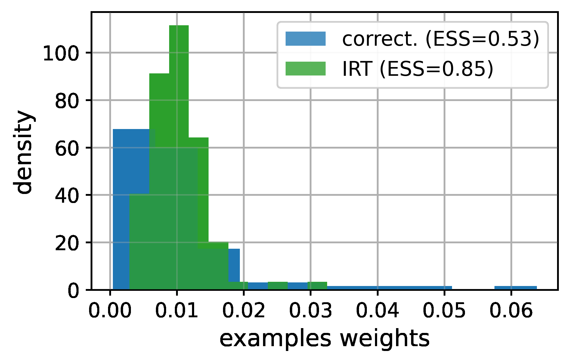
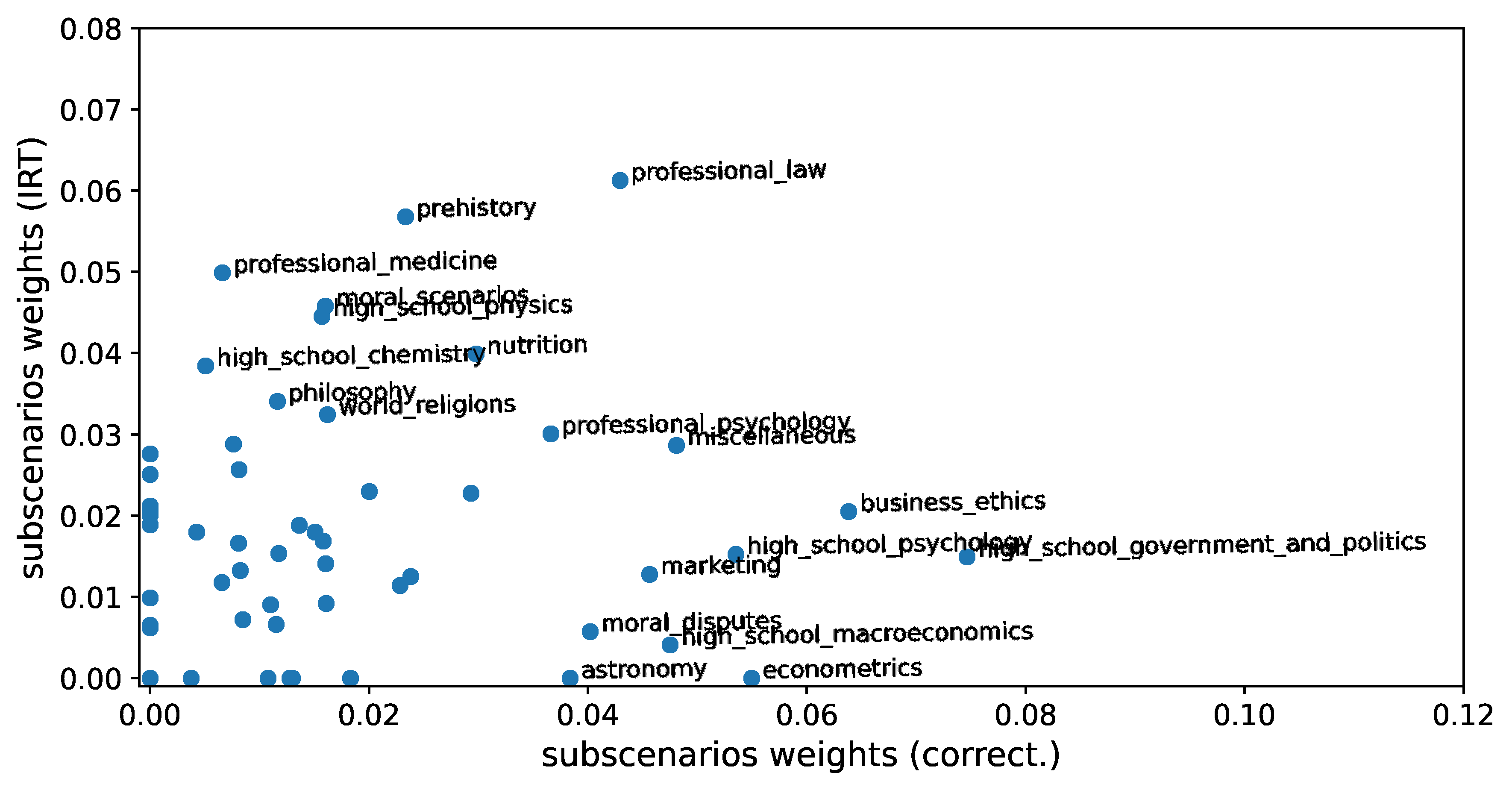
To better understand the composition of tinyMMLU, in Figure 9 we visualize the distribution of the weights of the selected examples and compare it to the weights of the correctness anchors. Recall that weights are non-negative and sum to 1. If an item has a weight 0.1, for example, that item has a contribution of 10% in the final estimated score. From Figure 9, we can see that tinyMMLU has more uniform weights compared to its correctness-based counterpart. We measure uniformity through the effective sample size (ESS) of the example weights. ESS, traditionally used in the Monte Carlo and domain adaptation (Elvira et al., 2022; Maia Polo & Vicente, 2023) literature, measures weight inequality in a way such that ESS = 0.50, for example, informally means that the corresponding weighted average is influenced by only 50% of (uniformly weighted) examples. In the context of our problem, more uniform weights of tinyMMLU contribute to its robustness when evaluating LLMs with varying correctness patterns, such as specialized LLMs in Figure 5. We also investigate the total weight of the tinyMMLU examples within each of the 57 subjects in Figure 10. The highest weighted are "high school psychology", "elementary mathematics", and "professional law". Interestingly the weight of the subjects is fairly different from its correctness-based counterpart.
为更好理解 tinyMMLU 的构成,图 9 可视化了所选示例权重的分布,并与 correctness 锚点的权重比较。回顾:权重非负且和为 1。例如,若某项目权重为 0.1,则该项目对最终估计得分的贡献为 10%。从图 9 可见,tinyMMLU 的权重比其 correctness 版本更均匀。我们用示例权重的有效样本量(effective sample size,ESS)度量均匀性。ESS 传统上用于蒙特卡洛与域适应文献(Elvira et al., 2022; Maia Polo & Vicente, 2023),度量权重不平等:例如 ESS = 0.50 非正式地意味着相应的加权平均只受到 50% 的(等权)示例影响。在我们问题的语境中,tinyMMLU 更均匀的权重有助于它在评测正确性模式各异的 LLM(如图 5 中的特化 LLM)时的鲁棒性。我们还在图 10 中考察了 tinyMMLU 示例在 57 个学科内部的总权重。总权重最高的是「高中心理学」(high school psychology)、「初等数学」(elementary mathematics)与「专业法律」(professional law)。有趣的是,各学科的权重与其 correctness 版本相当不同。
[图 9: Comparing the spread of examples weights using both the IRT and correctness approaches to find anchor points. We see that weights inequality is much higher when we cluster examples using correctness.]
图 9:比较用 IRT 与 correctness 两种方法找锚点时示例权重的分布。可以看到,用 correctness 聚类示例时,权重不平等要高得多。
[图 10: Weights given to MMLU subscenarios by the two anchoring methods.]
图 10:两种锚点方法给 MMLU 各子场景(57 个学科)分配的权重。
附录 C 命题 4.1 的证明(Proof of Proposition 4.1)
Proof of proposition 4.1. See that
|ˆE[Zjl|Yi0l,··· ,Yikl]− E[Zjl|Yi0l,··· ,Yikl]| ≤ (1−λˆ)/|Ij\Îj| Σi∈Ij\Îj |σ(ˆθ⊤l αi−βi)−σ(θ⊤l αi−βi)| ≤ 1/|Ij\Îj| Σi∈Ij\Îj |(ˆθl−θl)⊤αi| ≤ 1/|Ij\Îj| Σi∈Ij\Îj ∥αi∥2 ∥ˆθl−θl∥2 ≤ c∥ˆθl−θl∥2 → 0
in probability as |Î|→∞. The second step uses the fact that σ is 1/4-Lipschitz and the third step applies Cauchy-Schwarz inequality.
命题 4.1 的证明。见
(当 $|\hat I| \to \infty$ 时依概率)。第二步用了 $\sigma$ 为 1/4-Lipschitz 的事实,第三步应用 Cauchy-Schwarz 不等式。
附录 D 基准的更多细节(More details about benchmarks)
HuggingFace's Open LLM Leaderboard (Beeching et al., 2023): the data from this benchmark is composed of 395 LLMs and approx. 29k items that were downloaded from the platform in January/2024. To extract data from those models, we filter all models from the platform that have an MMLU score over 5.3, order them according to their average performance, and equally spaced selected models. Then, we kept all models that had scores for all six scenarios: ARC (Clark et al., 2018), HellaSwag (Zellers et al., 2019), MMLU (Hendrycks et al., 2020), TruthfulQA (Lin et al., 2021), Winogrande (Sakaguchi et al., 2021), and GSM8K (Cobbe et al., 2021). In a second round of data collection, we collected data for 40 "specialized models" by recognizing which models were fine-tuned to do the math, coding, etc.. The two sets of models have an intersection, and in total, we have collected data from 428 LLMs.
- HuggingFace 的 Open LLM Leaderboard(Beeching et al., 2023):该基准的数据由 395 个 LLM 与约 29K 个项目组成,于 2024 年 1 月从平台下载。为从这些模型提取数据,我们过滤出平台上 MMLU 分数超过 5.3 的所有模型(原文脚注 5:指排行榜上的分数。我们实际使用的分数可能不同,因为我们用的是对排行榜的最后一次提交,而排行榜展示的是所有提交中的最佳结果),按平均性能排序,并等距选取模型。然后,我们保留在全部六个场景上都有得分的模型:ARC(Clark et al., 2018)、HellaSwag(Zellers et al., 2019)、MMLU(Hendrycks et al., 2020)、TruthfulQA(Lin et al., 2021)、Winogrande(Sakaguchi et al., 2021)与 GSM8K(Cobbe et al., 2021)。第二轮数据收集中,我们通过识别哪些模型是为数学、代码等而微调的,收集了 40 个「特化模型」的数据。两组模型有交集,总计我们收集了 428 个 LLM 的数据。
HELM (Liang et al., 2022): we use HELM Lite (https://crfm.stanford.edu/helm/lite) v1.0.0, which is a dataset composed of 37 LLMs and approx. 10k evaluation examples from 10 scenarios. The scenarios are OpenbookQA (Mihaylov et al., 2018), MMLU (Hendrycks et al., 2020), NarrativeQA (Kočiský et al., 2018), NaturalQuestions (closed-book) (Kwiatkowski et al., 2019), NaturalQuestions (open-book), Math (Hendrycks et al., 2021), GSM8K (Cobbe et al., 2021), LegalBench (Guha et al., 2024), MedQA (Jin et al., 2021), WMT14 (Bojar et al., 2014).
- HELM(Liang et al., 2022):我们使用 HELM Lite(https://crfm.stanford.edu/helm/lite)v1.0.0——一个由 37 个 LLM 与来自 10 个场景的约 10K 个评测示例组成的数据集。这些场景是:OpenbookQA(Mihaylov et al., 2018)、MMLU(Hendrycks et al., 2020)、NarrativeQA(Kočiský et al., 2018)、NaturalQuestions(closed-book)(Kwiatkowski et al., 2019)、NaturalQuestions(open-book)、Math(Hendrycks et al., 2021)、GSM8K(Cobbe et al., 2021)、LegalBench(Guha et al., 2024)、MedQA(Jin et al., 2021)、WMT14(Bojar et al., 2014)。
附录 E 额外结果(Extra results)
E.1 更长时间跨度上预测性能的鲁棒性(Robustness in predicting performance in a longer time horizon)
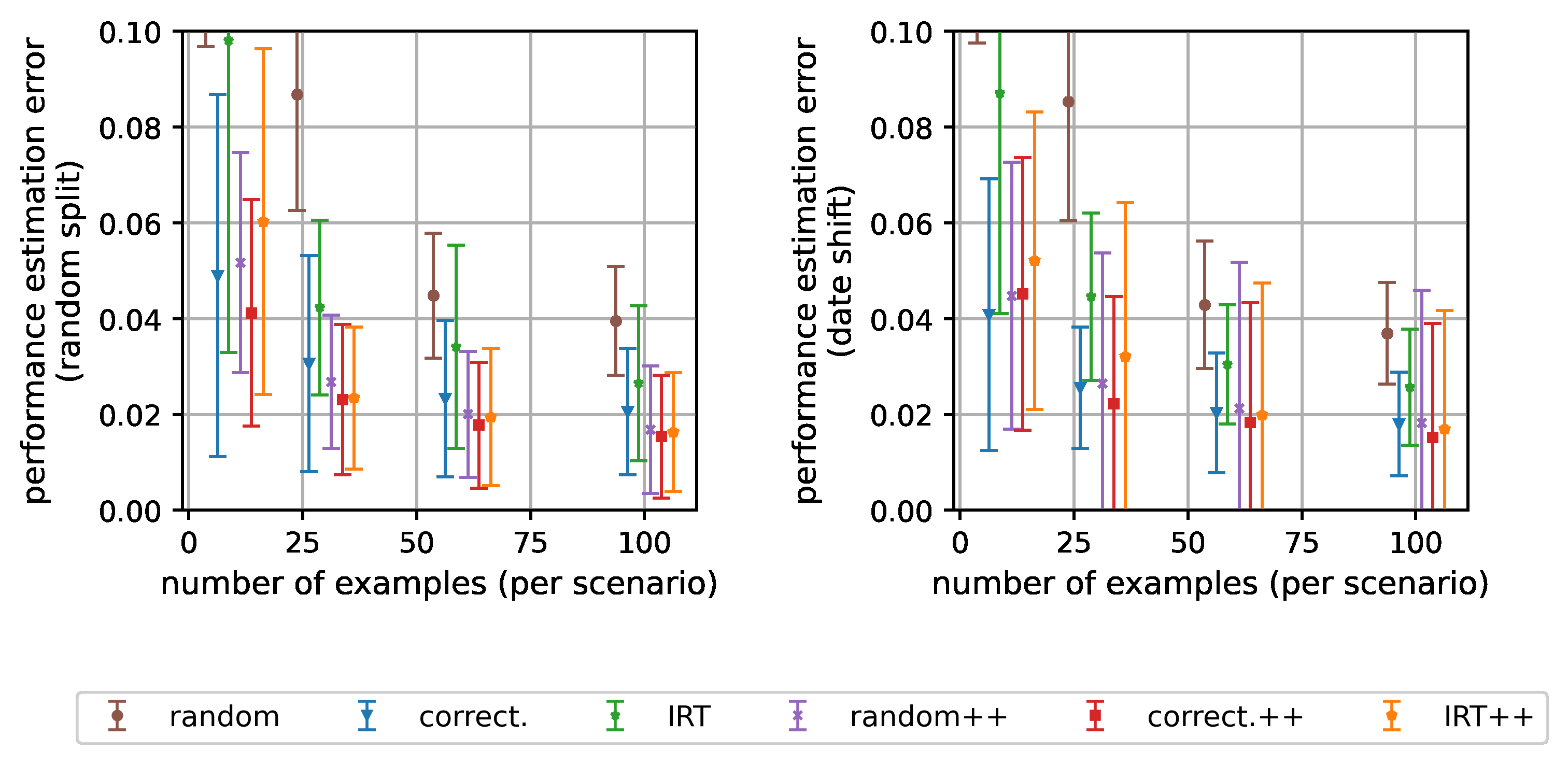
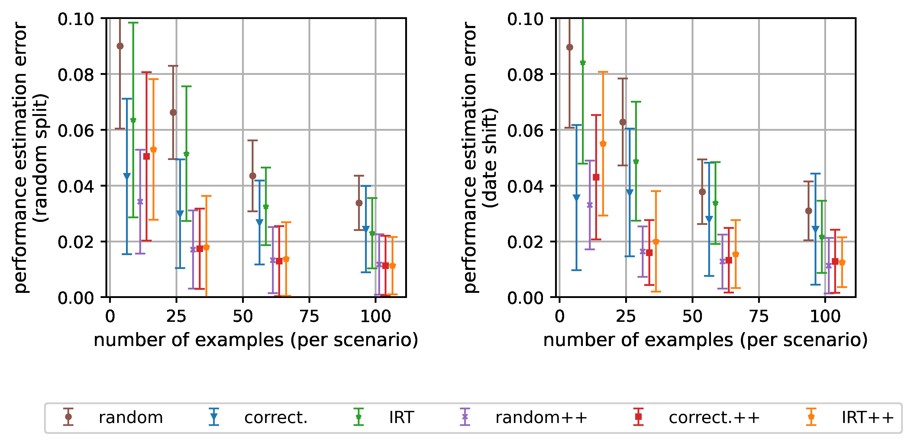
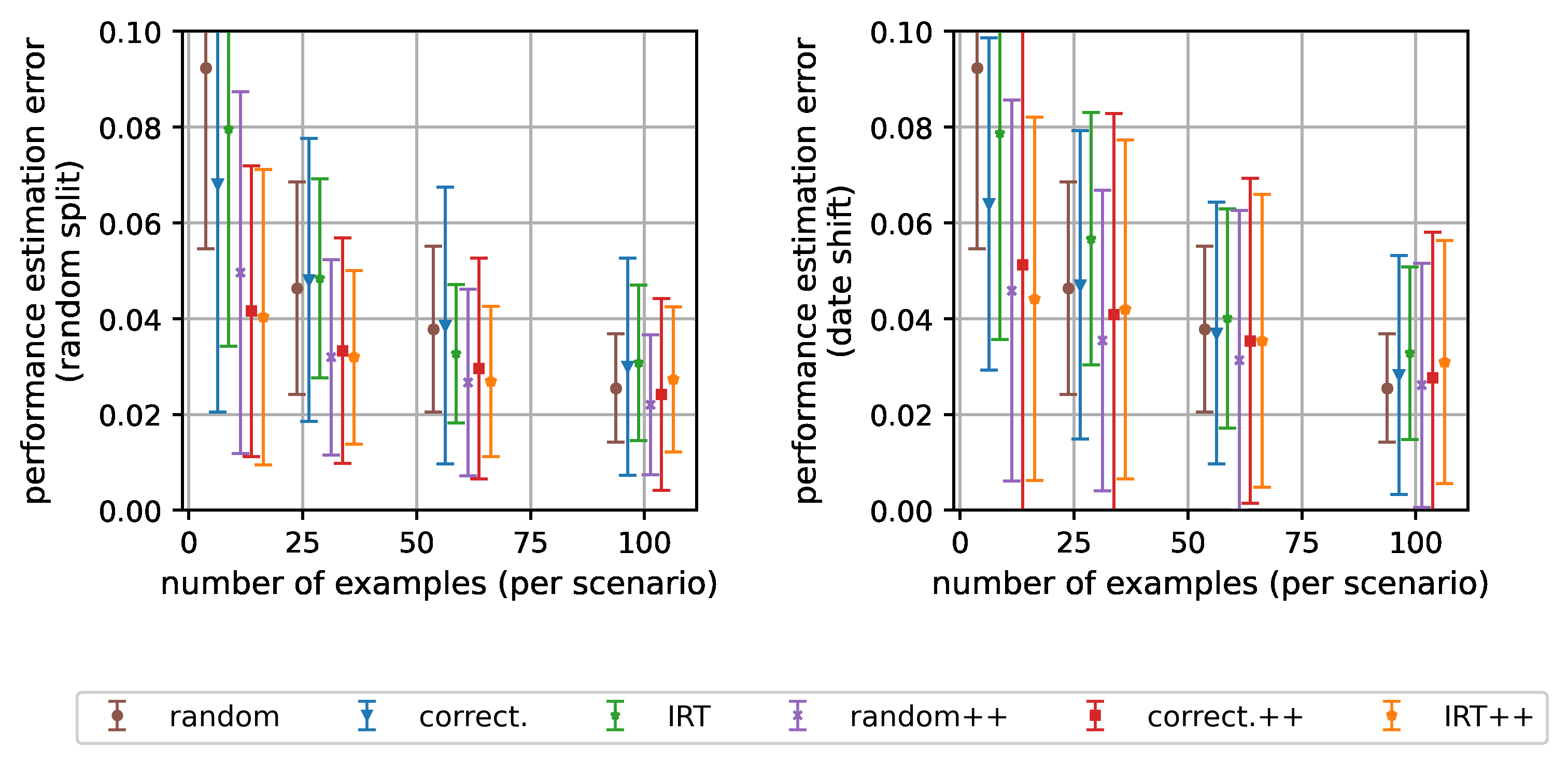
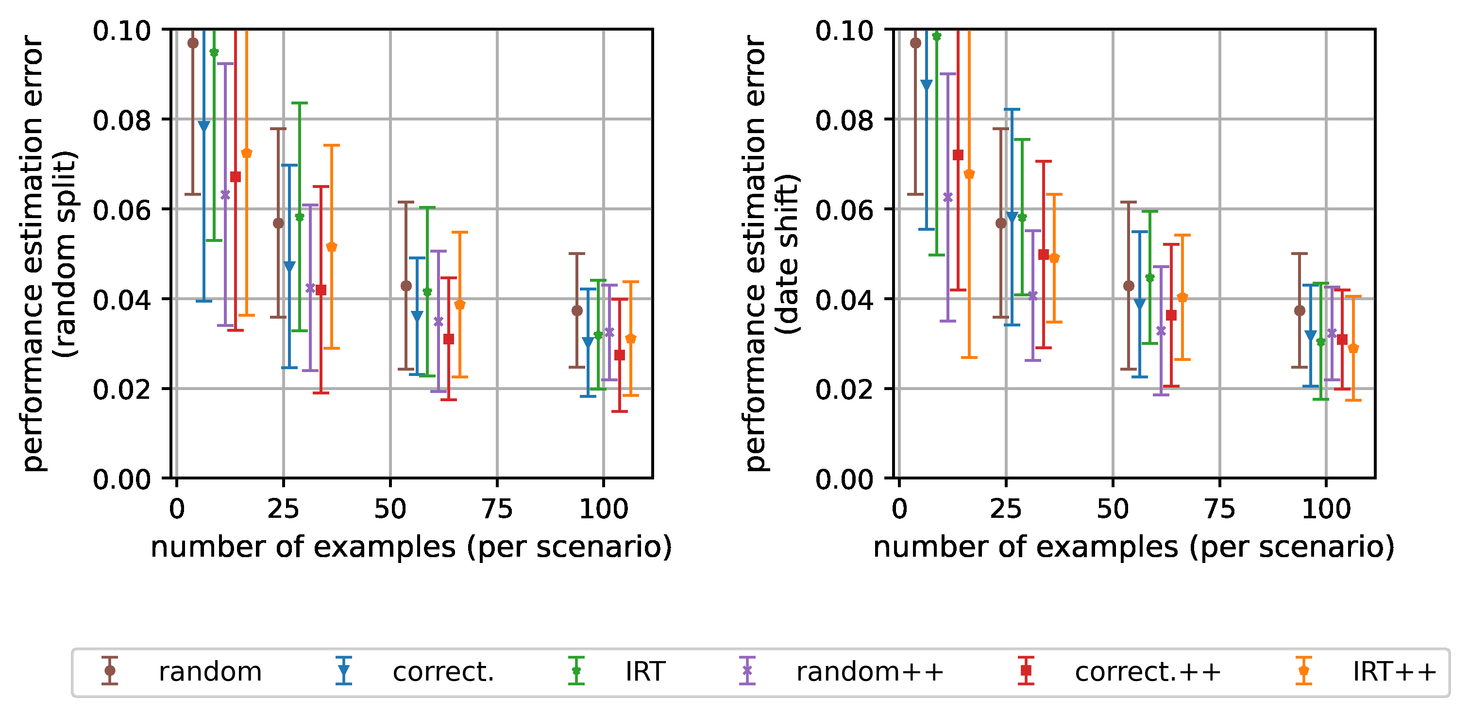
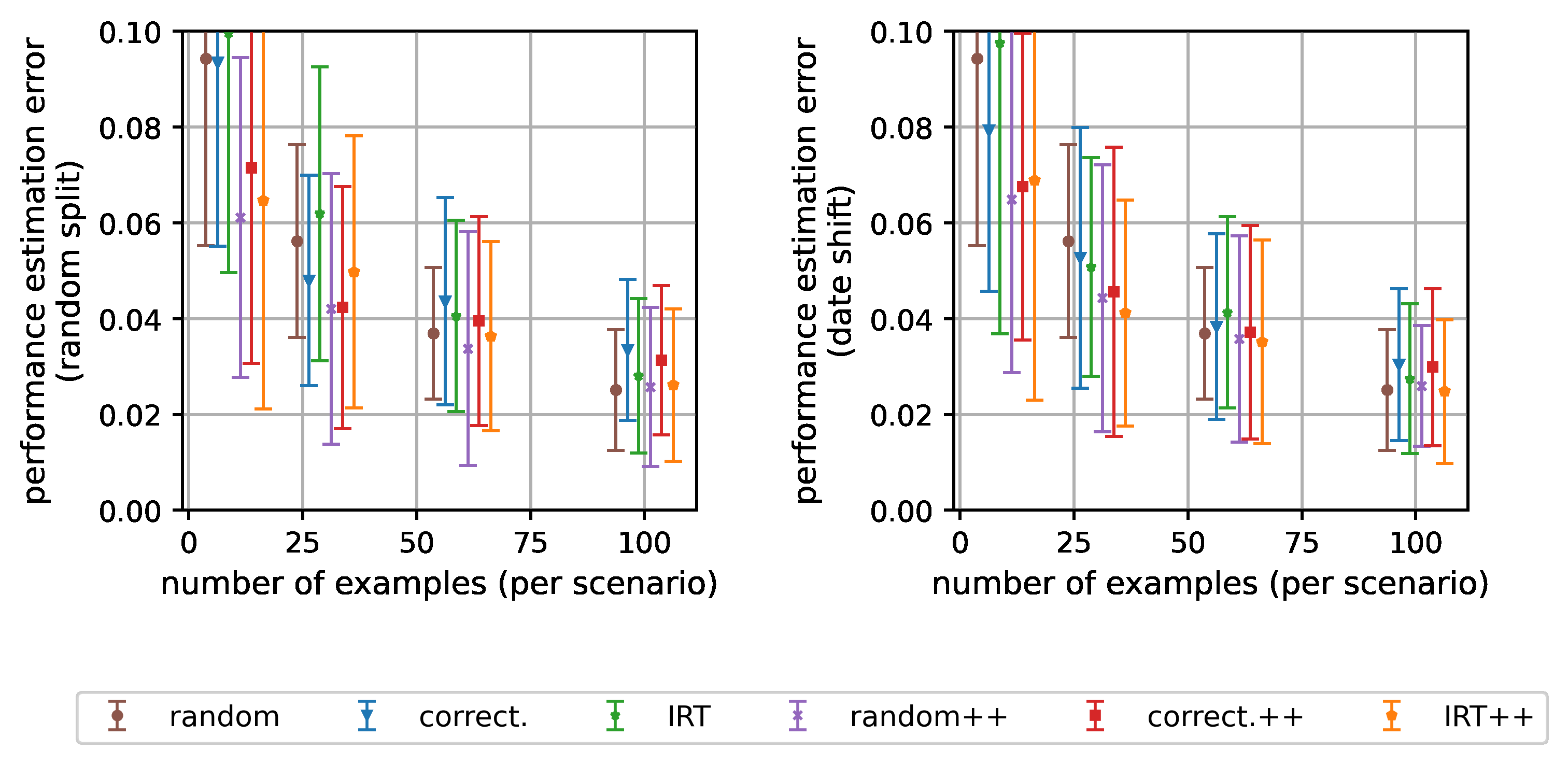
We conduct extra ablation studies placing 75% of the data in the test set. For the Open LLM Leaderboard and MMLU, it means we are using 3 months of future data as the test set (vs. approx. 3 weeks in the main text) while for AlpacaEval 2.0 that would correspond to 6 months (vs. approx. 2 months in the main text). In general, we show that our main method "IRT++" is pretty robust to the advancements in the field when predicting the performance of new LLMs. We report in the following plots the average estimation error in the test set (using 75% of the most recent data in the test set) and standard deviation across LLMs. The results do not differ considerably from the ones in the main text.
我们做了额外的消融研究,把 75% 的数据放进测试集。对 Open LLM Leaderboard 与 MMLU,这意味着用 3 个月的未来数据做测试集(正文约 3 周);对 AlpacaEval 2.0 相当于 6 个月(正文约 2 个月)。总体上,我们表明主方法「IRT++」在预测新 LLM 性能时对该领域的进展相当鲁棒。下列各图给出测试集(用最近 75% 的数据)上的平均估计误差以及跨 LLM 的标准差。结果与正文没有显著差别。
[图 11: Our methods are robust in predicting performance in a longer time horizon]
图 11:我们的方法在更长时间跨度上预测性能是鲁棒的(Open LLM Leaderboard、MMLU、AlpacaEval 三列,75% 按日期划分,随机/correct./IRT 及各 ++ 变体)。
E.2 分层随机抽样要用多大样本才能击败 IRT++?(How costly is it for stratified random sampling beat IRT++ with larger samples?)
We present results comparing IRT++ and stratified random sampling for a larger number of evaluation examples n. On Open LLM Leaderboard 400 examples per task (2400 total) are enough to match IRT++ with 100 examples per task (600 total). On MMLU, random sampling improves quite slowly and would require >400 examples to match IRT++ at 100. On AlpacaEval, random with 200 examples matches IRT++ with 100 examples (note that AlpacaEval is a small benchmark with 805 examples total, but evaluation requires GPT-4 and is thus quite expensive). We use the random split for the LLMs, implying no distribution shift between train and test.
我们给出 IRT++ 与分层随机抽样在更大评测示例数 $n$ 下的比较结果。在 Open LLM Leaderboard 上,每任务 400 例(共 2400)足以追平 IRT++ 每任务 100 例(共 600);在 MMLU 上,随机抽样改进得相当慢,需要超过 400 例才能追平 IRT++ 的 100 例;在 AlpacaEval 上,随机 200 例追平 IRT++ 的 100 例(注意 AlpacaEval 是总共 805 例的小基准,但评测需要 GPT-4,因此相当昂贵)。我们对 LLM 用随机划分,即训练与测试之间无分布偏移。
[图 12: Benchmark results for different methods and sample sizes]
图 12:不同方法与样本量下的基准结果(每场景/基准 100–400 例,iid 划分)。
E.3 运行时间(Running time)
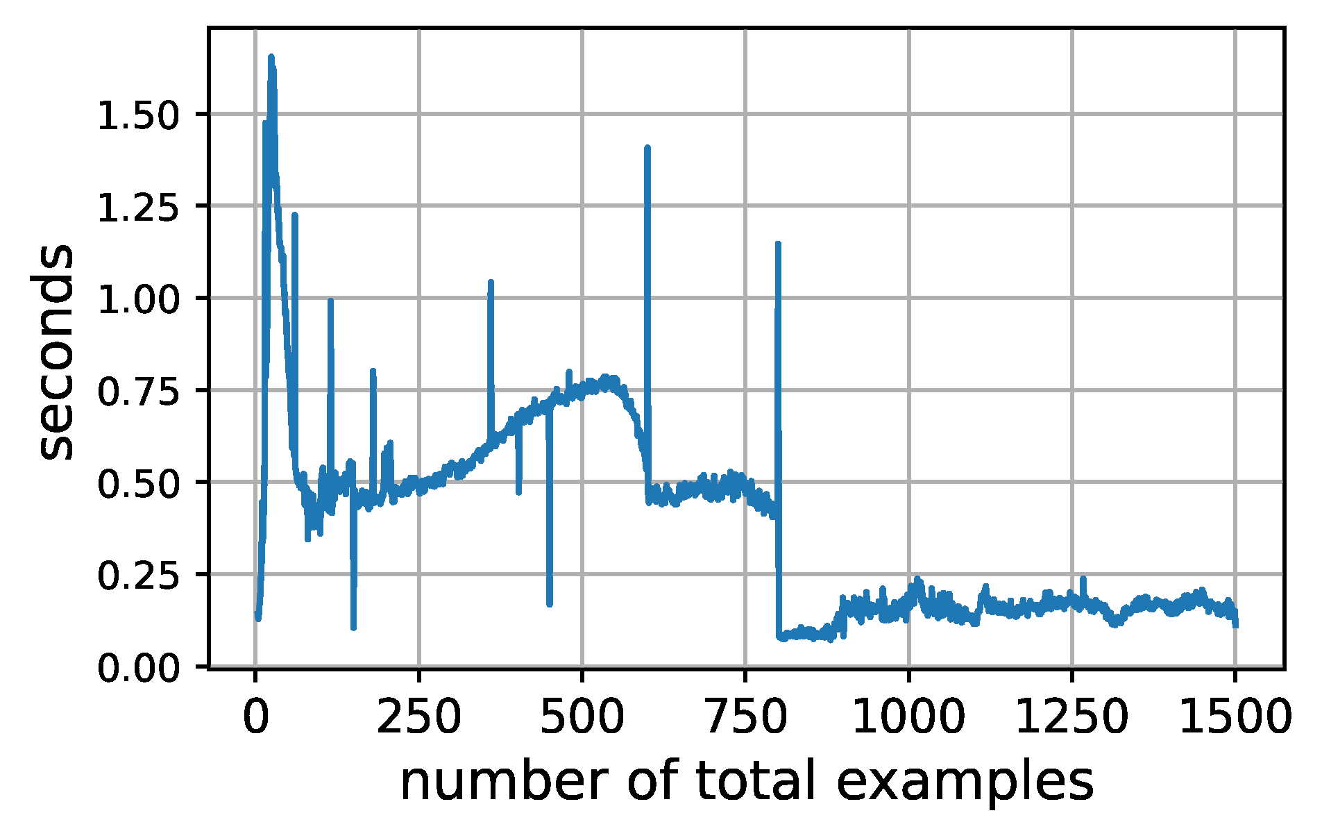
We record the running time of IRT inference (ability parameter fitting) when running our experiments. In Figure 13 we show that the average running time is fairly negligible.
我们记录了实验中 IRT 推断(能力参数拟合)的运行时间。图 13 表明平均运行时间相当可忽略。
[图 13: Average running time by the amount of test examples: IRT inference.]
图 13:IRT 推断的平均运行时间随测试示例数量的变化:平均仅数秒,基本可忽略。
E.4 秩相关结果(Rank correlation results)
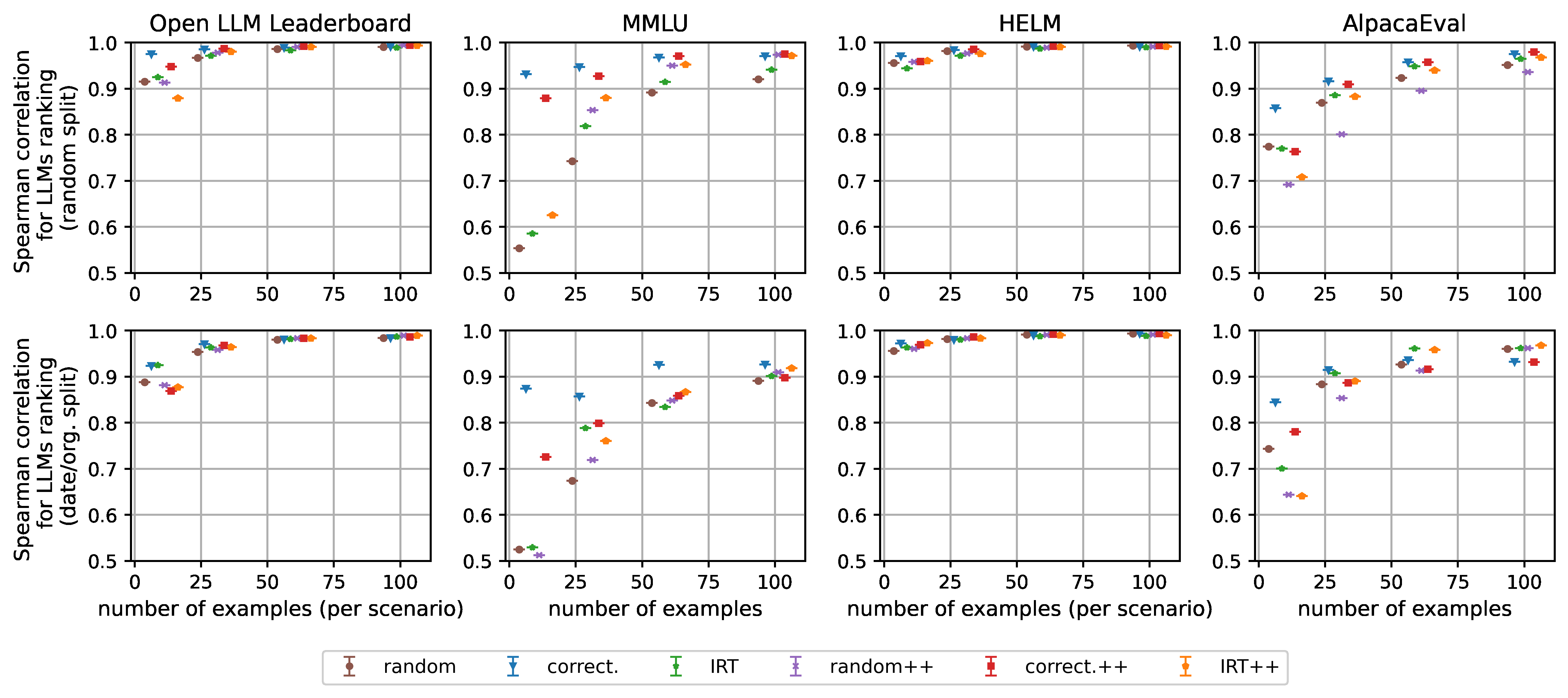
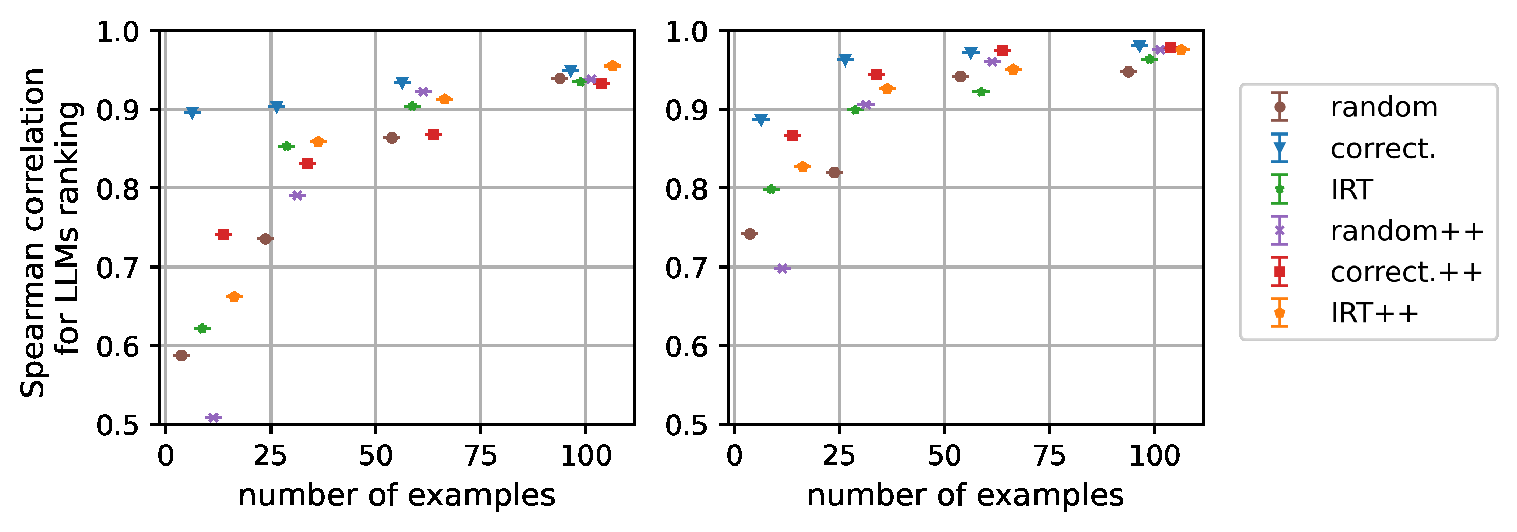
In this section, we explore versions of Figures 3 and 5 when we look at rank correlation (correlation between true and predicted ranking) instead of performance. It is clear from the plots below that our method can be used to rank models efficiently with tiny samples.
本节给出图 3 与图 5 改看秩相关(rank correlation,真实排名与预测排名之间的相关)而非性能的版本。从下图清晰可见:我们的方法可用微小样本高效地为模型排序。
[图 14: Rank correlation for true performance and predicted performance among LLMs.]
图 14:各 LLM 真实性能与预测性能之间的秩相关(对应图 3 的版本)。
[图 15: Rank correlation for true performance and predicted performance among LLMs in MMLU. The plot on the left represents a random split of the data while the plot on the right considers specialized models as the test set.]
图 15:MMLU 上各 LLM 真实性能与预测性能之间的秩相关。左图为数据的随机划分,右图以特化模型为测试集(对应图 5 的版本)。
E.5 自适应测试(Adaptive testing)
In this section, we complement the results shown in Figure 8 for all benchmarks.
本节补全图 8 所示结果到所有基准。
[图 16: Results of adaptive testing for different benchmarks.]
图 16:不同基准(Open LLM Leaderboard、MMLU、HELM、AlpacaEval)上自适应测试的结果,每场景 25–100 例、无分布偏移划分下比较 random、IRT、IRT++ 与 adaptIRT++。
附录 F 各场景的个体表现(Individual performances per scenario)
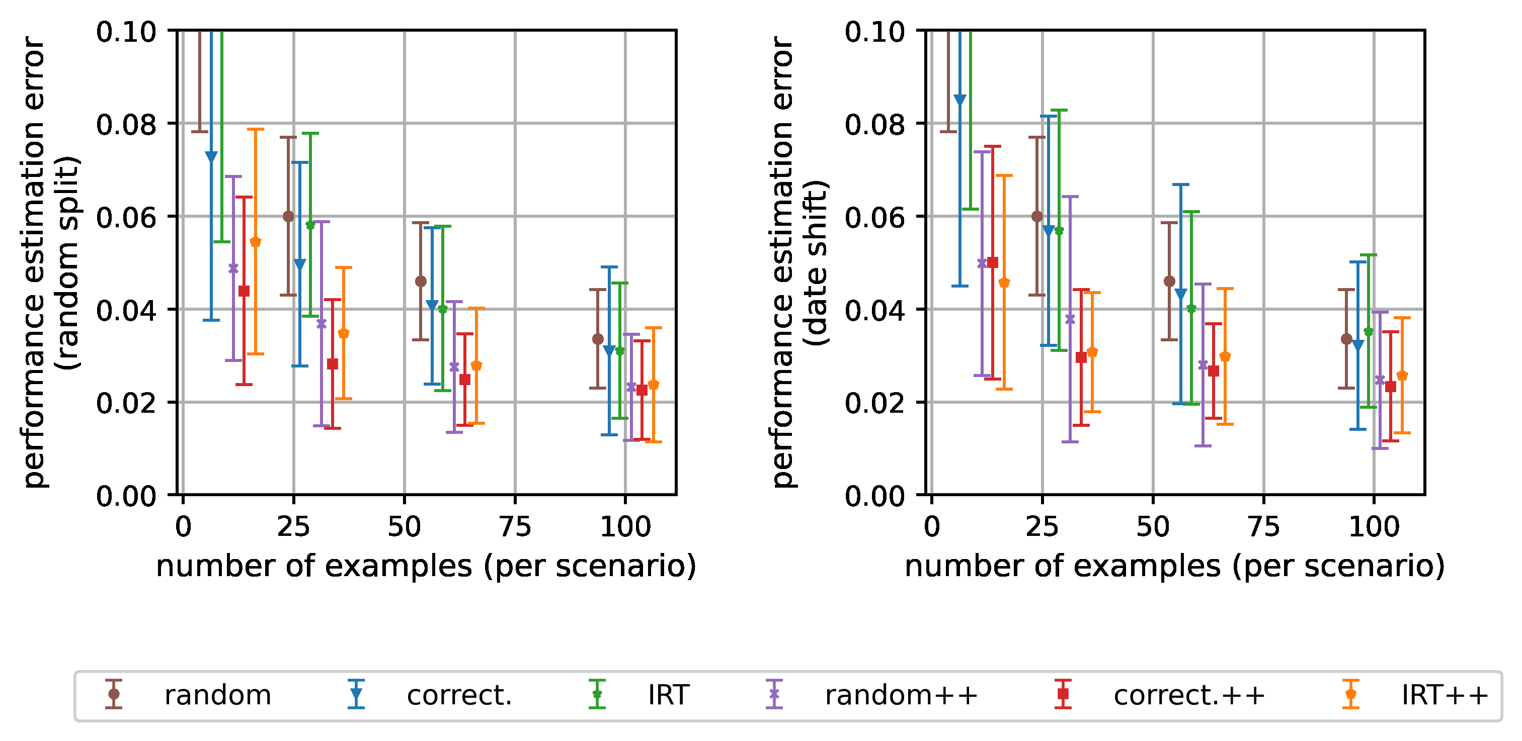
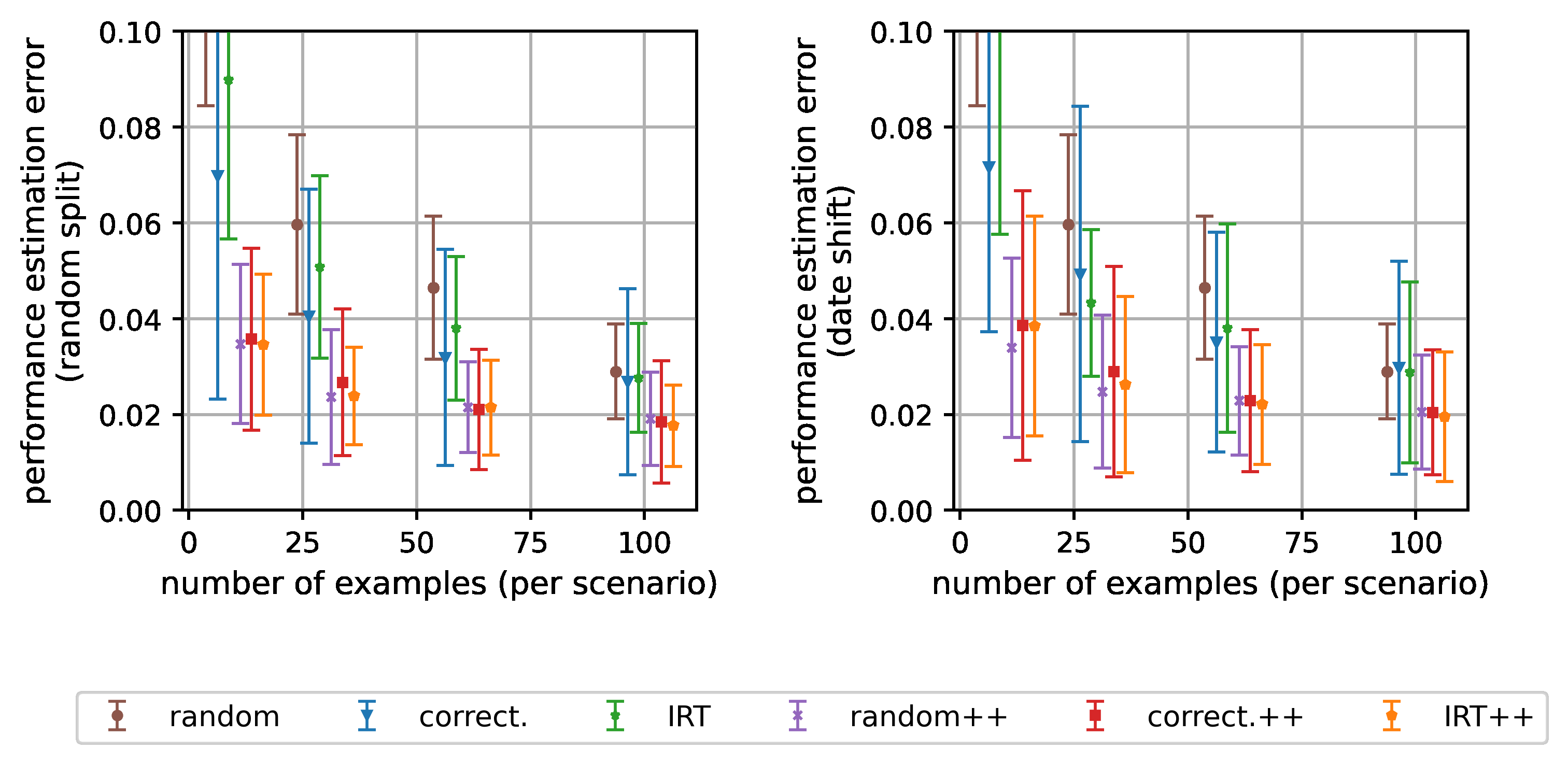
In this section, we explore what is behind Figure 3 by looking in detail at results for individual scenarios for the Open LLM Leaderboard and HELM. It is clear from the following plots that there are scenarios in which our methods shine more than others.
本节通过细看 Open LLM Leaderboard 与 HELM 各单独场景的结果,来探究图 3 背后的细节。从下列各图清晰可见:有些场景中我们的方法比在其他场景中更加出彩。
(译注:附录 F 其余部分仅由图 17–32 组成,无正文文字——图 17–22 依次为 Open LLM Leaderboard 的 ARC、GSM8K、TruthfulQA、HellaSwag、MMLU、Winogrande 六个场景的逐场景误差曲线;图 23–32 依次为 HELM 的 OpenbookQA、GSM、LegalBench、Math、MedQA、MMLU、NarrativeQA、NaturalQA(closed book)、NaturalQA(open book)、WMT14 十个场景的同类曲线。各图图题即场景名,故不逐图收录,请查阅原文 PDF。)
要点速览
- 动机:基准数万示例使评测极贵(HELM 全量评测一个模型 >4K GPU 小时 / >$10K API 费),而检查点监控与提示/超参探索需要反复评测——需要「用更少示例估计全基准性能」的方法。
- 方法总览:三类选例策略(分层随机抽样、correctness 聚类锚点、IRT 聚类锚点)× 两个估计变体(朴素加权平均、gp-IRT 校正),共六种;历史全量评测数据用于找锚点与拟合 IRT。
- IRT 建模:把 LLM 当考生、题目当试题,p_il = σ(α_iᵀθ_l − β_i);θ_l 是模型能力、α_i 是题目所需能力、β_i 是难度偏置;题目表示 (α̂_i, β̂_i) 低维(≤16),天然适合聚类找锚点。
- gp-IRT 估计器:加权的锚点估计(低偏差、高方差)与 p-IRT 预测(低方差、可能有偏)的凸组合,权重 λ = b̂²/(σ̂²/|Î_j|+b̂²) 由估计偏差与样本量自动决定;非二值得分先按阈值 c 二值化再建模。
- 核心数字:每场景 100 题即可把估计误差压到约 2%——MMLU 14K→100(降本 140 倍)、Open LLM Leaderboard 每场景 30 题就够(29K→180,降 160 倍)、HELM 10K→1,000、AlpacaEval 805→100。
- 鲁棒性:按日期用最新模型测试(时间偏移)依然有效;40 个领域特化 LLM 上 correctness 锚点明显退化而 IRT 锚点几乎不受影响;单模型误差几乎都 ≤4%;把测试集扩到 6 个月未来数据结论不变。
- 发布物:Open LLM Leaderboard、MMLU、HELM、AlpacaEval 2.0 的 tiny 版本(每场景 100 题)+ gp-IRT 工具(代码与预训练 IRT 参数,CPU 数秒),配合 HuggingFace 数据与 Colab 演示。
- 扩展:方法可迁移到提示评测(跨模板、跨模型规模偏移下仍准)与自适应选题(误差更低但当前实现需 5 分钟以上)。
- 局限与对策:严重分布偏移(如「简单题错、难题对」的异常模式)与模型能力快速跃升会损害外推;应定期用新模型数据更新精选题目与 IRT 参数。
- 课程关联:与 Press 的基准设计帖(怎么造)、Zhu2025 的严谨性检查清单(怎么查)构成评测单元三步曲;本文回答「怎么便宜可靠地评」,其「锚点+统计模型」思路也可迁移到 Agent 基准的成本控制。
🖼 原文图表(25 张)—— 提取自原始文献,点击展开
以上图片提取自原始 PDF/网页或 arXiv 官方 HTML 版(含矢量图与原始图注),已镜像至本站;与正文的对应关系请以原文为准。